Simple Linear Regression

Prof. Maria Tackett

Aug 31, 2022

Announcements

Meet your neighbor

Take a few moments to meet or (reconnect with) your neighbor!

  • Name
  • Year
  • Major
  • A highlight or something that stood out in the first two days of class
03:00

Data science life cycle from R for Data Science with modifications from The Art of Statistics: How to Learn from Data.

Topics

  • Use simple linear regression to describe the relationship between a quantitative predictor and quantitative response variable.

  • Estimate the slope and intercept of the regression line using the least squares method.

  • Interpret the slope and intercept of the regression line.

  • Predict the response given a value of the predictor variable.

  • Defined extrapolation and why we should avoid it.

Computation set up

# load packages
library(tidyverse)       # for data wrangling
library(tidymodels)      # for modeling
library(fivethirtyeight) # for the fandango dataset

# set default theme and larger font size for ggplot2
ggplot2::theme_set(ggplot2::theme_bw(base_size = 16))

# set default figure parameters for knitr
knitr::opts_chunk$set(
  fig.width = 8,
  fig.asp = 0.618,
  fig.retina = 3,
  dpi = 300,
  out.width = "80%"
)

Data

Movie ratings

Fandango logo

IMDB logo

Rotten Tomatoes logo

Metacritic logo

Data prep

  • Rename Rotten Tomatoes columns as critics and audience
  • Rename the dataset as movie_scores
movie_scores <- fandango |>
  rename(critics = rottentomatoes, 
         audience = rottentomatoes_user)

Data overview

glimpse(movie_scores)
Rows: 146
Columns: 23
$ film                       <chr> "Avengers: Age of Ultron", "Cinderella", "A…
$ year                       <dbl> 2015, 2015, 2015, 2015, 2015, 2015, 2015, 2…
$ critics                    <int> 74, 85, 80, 18, 14, 63, 42, 86, 99, 89, 84,…
$ audience                   <int> 86, 80, 90, 84, 28, 62, 53, 64, 82, 87, 77,…
$ metacritic                 <int> 66, 67, 64, 22, 29, 50, 53, 81, 81, 80, 71,…
$ metacritic_user            <dbl> 7.1, 7.5, 8.1, 4.7, 3.4, 6.8, 7.6, 6.8, 8.8…
$ imdb                       <dbl> 7.8, 7.1, 7.8, 5.4, 5.1, 7.2, 6.9, 6.5, 7.4…
$ fandango_stars             <dbl> 5.0, 5.0, 5.0, 5.0, 3.5, 4.5, 4.0, 4.0, 4.5…
$ fandango_ratingvalue       <dbl> 4.5, 4.5, 4.5, 4.5, 3.0, 4.0, 3.5, 3.5, 4.0…
$ rt_norm                    <dbl> 3.70, 4.25, 4.00, 0.90, 0.70, 3.15, 2.10, 4…
$ rt_user_norm               <dbl> 4.30, 4.00, 4.50, 4.20, 1.40, 3.10, 2.65, 3…
$ metacritic_norm            <dbl> 3.30, 3.35, 3.20, 1.10, 1.45, 2.50, 2.65, 4…
$ metacritic_user_nom        <dbl> 3.55, 3.75, 4.05, 2.35, 1.70, 3.40, 3.80, 3…
$ imdb_norm                  <dbl> 3.90, 3.55, 3.90, 2.70, 2.55, 3.60, 3.45, 3…
$ rt_norm_round              <dbl> 3.5, 4.5, 4.0, 1.0, 0.5, 3.0, 2.0, 4.5, 5.0…
$ rt_user_norm_round         <dbl> 4.5, 4.0, 4.5, 4.0, 1.5, 3.0, 2.5, 3.0, 4.0…
$ metacritic_norm_round      <dbl> 3.5, 3.5, 3.0, 1.0, 1.5, 2.5, 2.5, 4.0, 4.0…
$ metacritic_user_norm_round <dbl> 3.5, 4.0, 4.0, 2.5, 1.5, 3.5, 4.0, 3.5, 4.5…
$ imdb_norm_round            <dbl> 4.0, 3.5, 4.0, 2.5, 2.5, 3.5, 3.5, 3.5, 3.5…
$ metacritic_user_vote_count <int> 1330, 249, 627, 31, 88, 34, 17, 124, 62, 54…
$ imdb_user_vote_count       <int> 271107, 65709, 103660, 3136, 19560, 39373, …
$ fandango_votes             <int> 14846, 12640, 12055, 1793, 1021, 397, 252, …
$ fandango_difference        <dbl> 0.5, 0.5, 0.5, 0.5, 0.5, 0.5, 0.5, 0.5, 0.5…

Movie ratings data

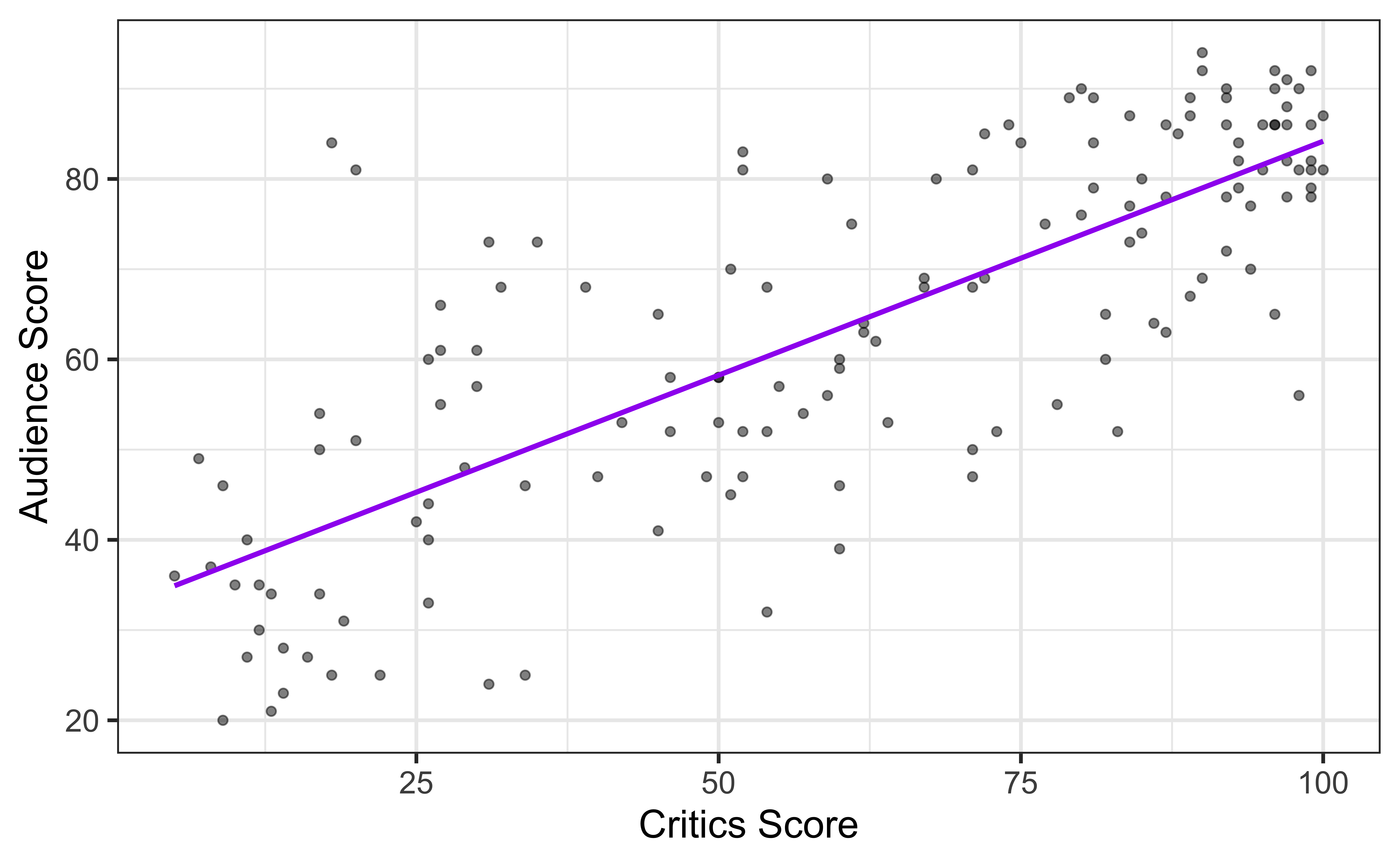
The data set contains the “Tomatometer” score (critics) and audience score (audience) for 146 movies rated on rottentomatoes.com.

Movie ratings data

Goal: Fit a line to describe the relationship between the critics score and audience score.

Why fit a line?

We fit a line to accomplish one or both of the following:

Prediction

What is the audience score expected to be for an upcoming movie that received 35% from the critics?

Inference

Is the critics score a useful predictor of the audience score? By how much is the audience score expected to change for each additional point in the critics score?

Terminology

  • Response, Y: variable describing the outcome of interest

  • Predictor, X: variable we use to help understand the variability in the response

Regression model

A regression model is a function that describes the relationship between the response, \(Y\), and the predictor, \(X\).

\[\begin{aligned} Y &= \color{black}{\textbf{Model}} + \text{Error} \\[8pt] &= \color{black}{\mathbf{f(X)}} + \epsilon \\[8pt] &= \color{black}{\boldsymbol{\mu_{Y|X}}} + \epsilon \end{aligned}\]

Regression model

\[\begin{aligned} Y &= \color{purple}{\textbf{Model}} + \text{Error} \\[8pt] &= \color{purple}{\mathbf{f(X)}} + \epsilon \\[8pt] &= \color{purple}{\boldsymbol{\mu_{Y|X}}} + \epsilon \end{aligned}\]

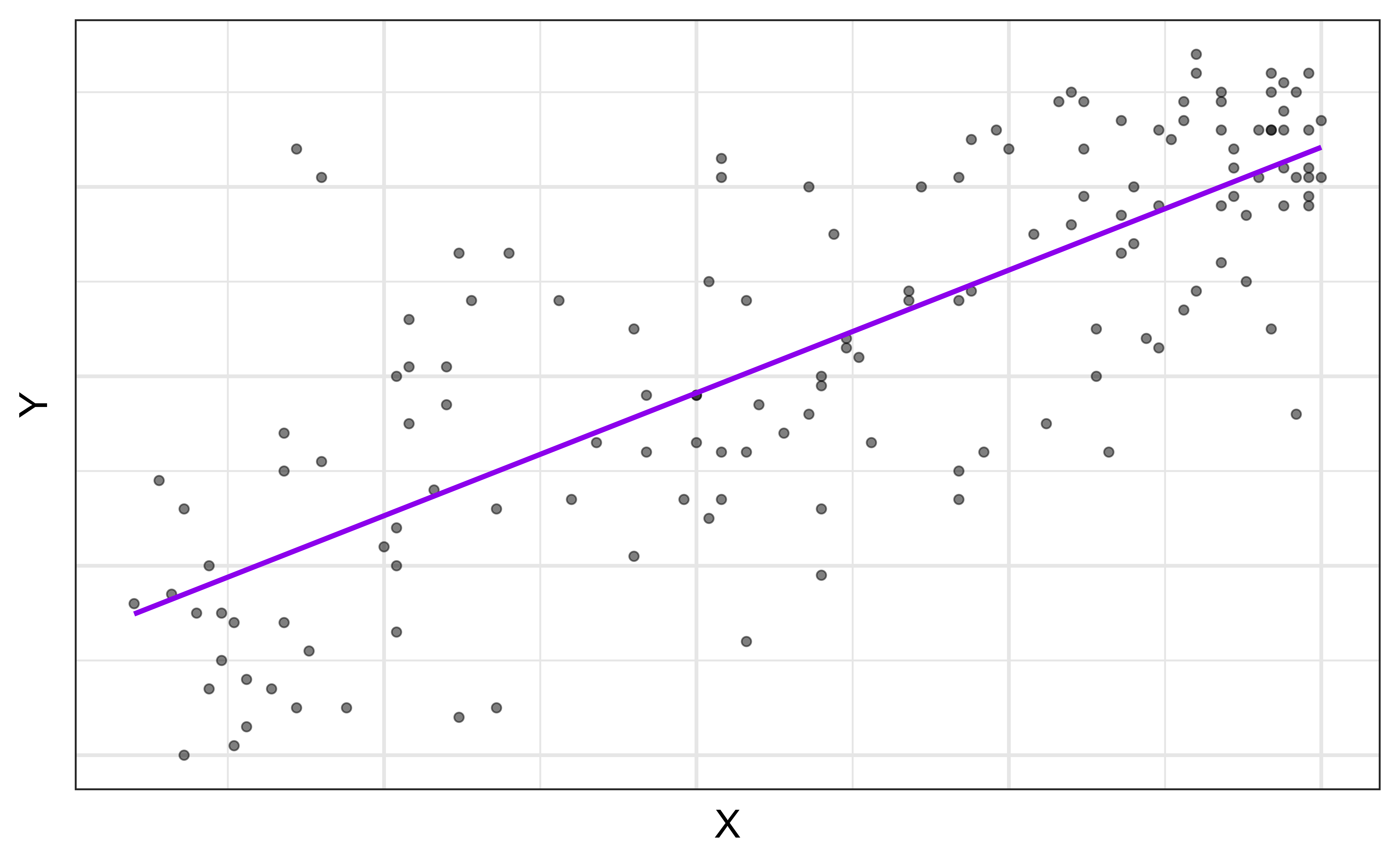
\(\mu_{Y|X}\) is the mean value of \(Y\) given a particular value of \(X\).

Regression model

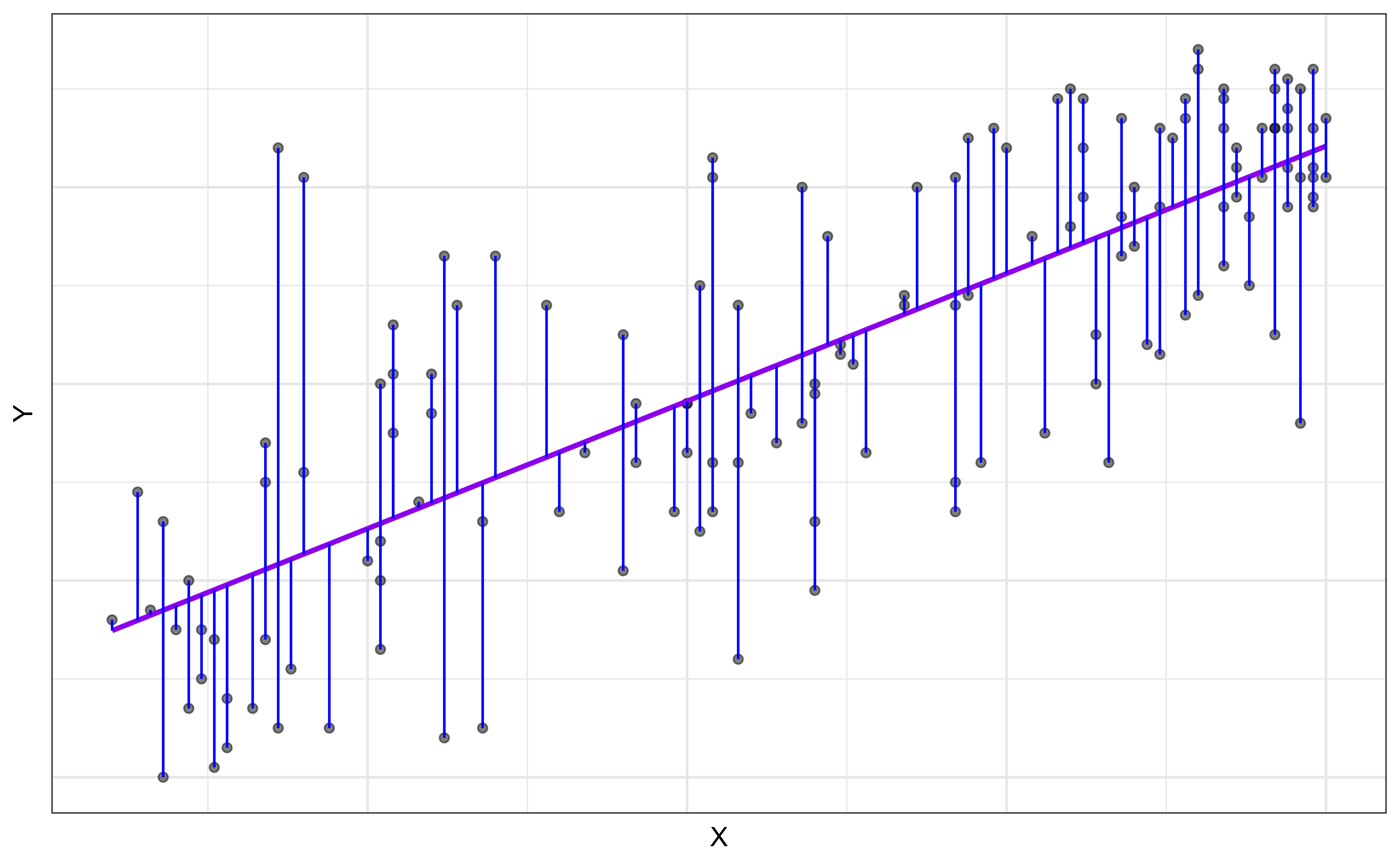
\[ \begin{aligned} Y &= \color{purple}{\textbf{Model}} + \color{blue}{\textbf{Error}} \\[5pt] &= \color{purple}{\mathbf{f(X)}} + \color{blue}{\boldsymbol{\epsilon}} \\[5pt] &= \color{purple}{\boldsymbol{\mu_{Y|X}}} + \color{blue}{\boldsymbol{\epsilon}} \\[5pt] \end{aligned} \]

Simple linear regression

Simple linear regression

When we have a quantitative response, \(Y\), and a single quantitative predictor, \(X\), we can use a simple linear regression model to describe the relationship between \(Y\) and \(X\). \[\Large{Y = \mathbf{\beta_0 + \beta_1 X} + \epsilon}\]

  • \(\beta_1\): True slope of the relationship between \(X\) and \(Y\)
  • \(\beta_0\): True intercept of the relationship between \(X\) and \(Y\)
  • \(\epsilon\): Error

Simple linear regression

\[\Large{\hat{Y} = \hat{\beta}_0 + \hat{\beta}_1 X}\]

  • \(\hat{\beta}_1\): Estimated slope of the relationship between \(X\) and \(Y\)
  • \(\hat{\beta}_0\): Estimated intercept of the relationship between \(X\) and \(Y\)
  • No error term!

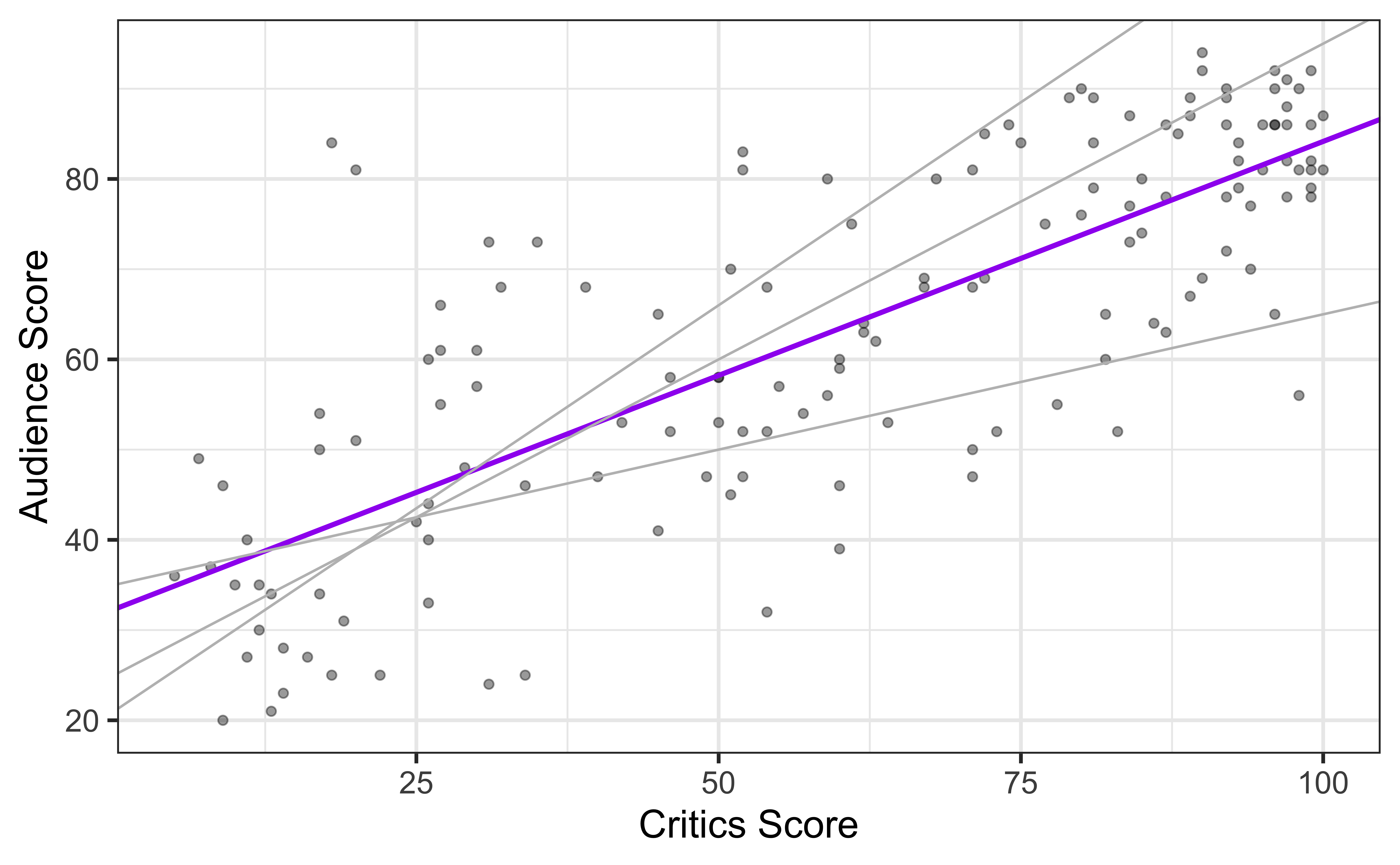
Choosing values for \(\hat{\beta}_1\) and \(\hat{\beta}_0\)

Residuals

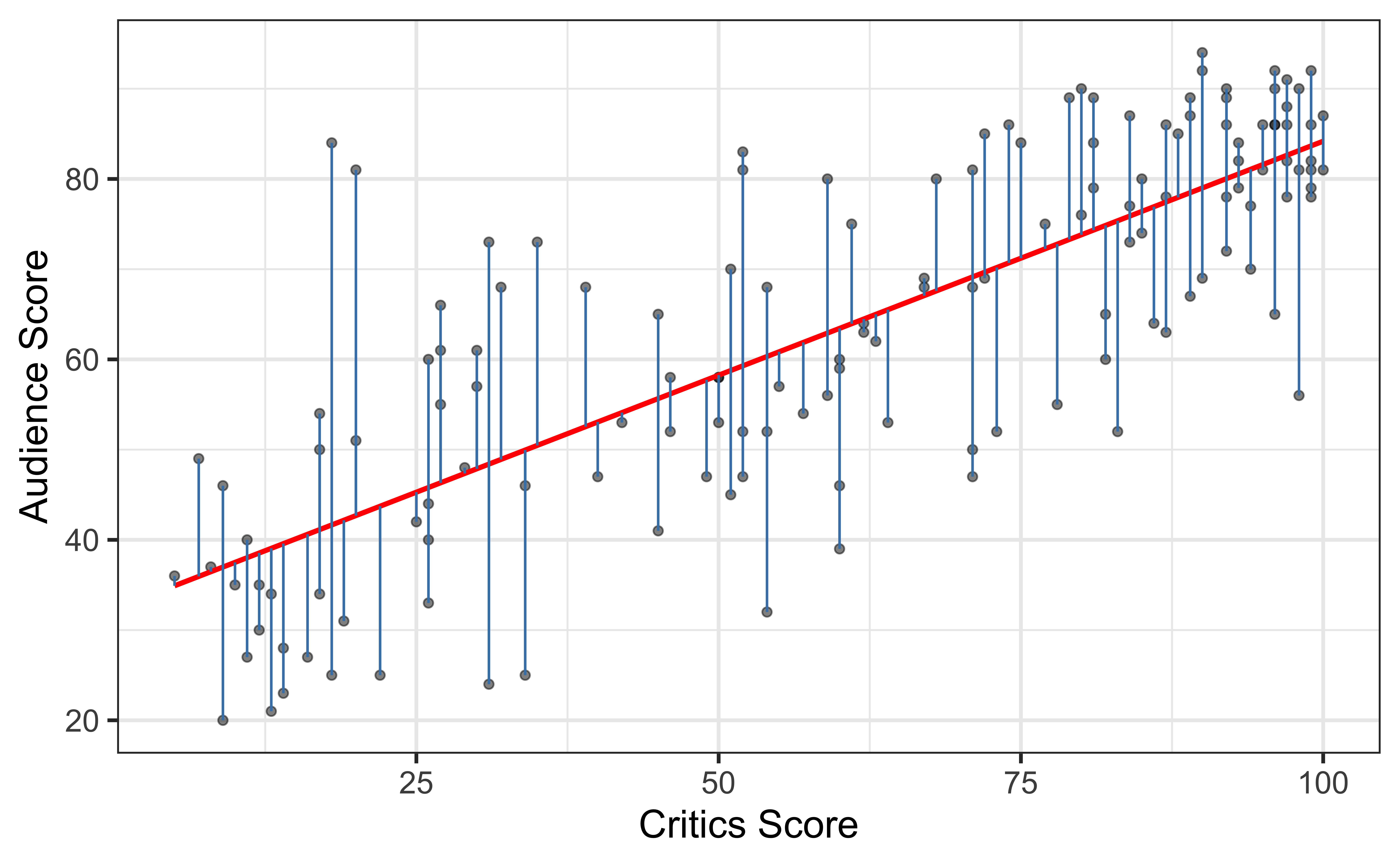
\[\text{residual} = \text{observed} - \text{predicted} = y - \hat{y}\]

Least squares line

  • The residual for the \(i^{th}\) observation is

\[e_i = \text{observed} - \text{predicted} = y_i - \hat{y}_i\]

  • The sum of squared residuals is

\[e^2_1 + e^2_2 + \dots + e^2_n\]

  • The least squares line is the one that minimizes the sum of squared residuals

Slope and intercept

Properties of least squares regression

  • The regression line goes through the center of mass point, the coordinates corresponding to average \(X\) and average \(Y\): \(\hat{\beta}_0 = \bar{Y} - \hat{\beta}_1\bar{X}\)

  • The slope has the same sign as the correlation coefficient: \(\hat{\beta}_1 = r \frac{s_Y}{s_X}\)

  • The sum of the residuals is zero: \(\sum_{i = 1}^n \epsilon_i = 0\)

  • The residuals and \(X\) values are uncorrelated

Estimating the slope

\[\large{\hat{\beta}_1 = r \frac{s_Y}{s_X}}\]

\[\begin{aligned} s_X &= 30.1688 \\ s_Y &= 20.0244 \\ r &= 0.7814 \end{aligned}\]
\[\begin{aligned} \hat{\beta}_1 &= 0.7814 \times \frac{20.0244}{30.1688} \\ &= 0.5187\end{aligned}\]


Click here for details on deriving the equations for slope and intercept.

Estimating the intercept

\[\large{\hat{\beta}_0 = \bar{Y} - \hat{\beta}_1\bar{X}}\]

\[\begin{aligned} &\bar{x} = 60.8493 \\ &\bar{y} = 63.8767 \\ &\hat{\beta}_1 = 0.5187 \end{aligned}\]
\[\begin{aligned}\hat{\beta}_0 &= 63.8767 - 0.5187 \times 60.8493 \\ &= 32.3142 \end{aligned}\]


Click here for details on deriving the equations for slope and intercept.

Interpretation

Post your answers to the following questions on Ed Discussion:

  • The slope of the model for predicting audience score from critics score is 0.5187 . Which of the following is the best interpretation of this value?

  • 32.3142 is the predicted mean audience score for what type of movies?

03:00

Does it make sense to interpret the intercept?

The intercept is meaningful in the context of the data if

  • the predictor can feasibly take values equal to or near zero, or

  • there are values near zero in the observed data.

🛑 Otherwise, the intercept may not be meaningful!

Prediction

Making a prediction

Suppose that a movie has a critics score of 70. According to this model, what is the movie’s predicted audience score?

\[\begin{aligned} \widehat{\text{audience}} &= 32.3142 + 0.5187 \times \text{critics} \\ &= 32.3142 + 0.5187 \times 70 \\ &= 68.6232 \end{aligned}\]

⚠️ Extrapolation

Using the model to predict for values outside the range of the original data is extrapolation.

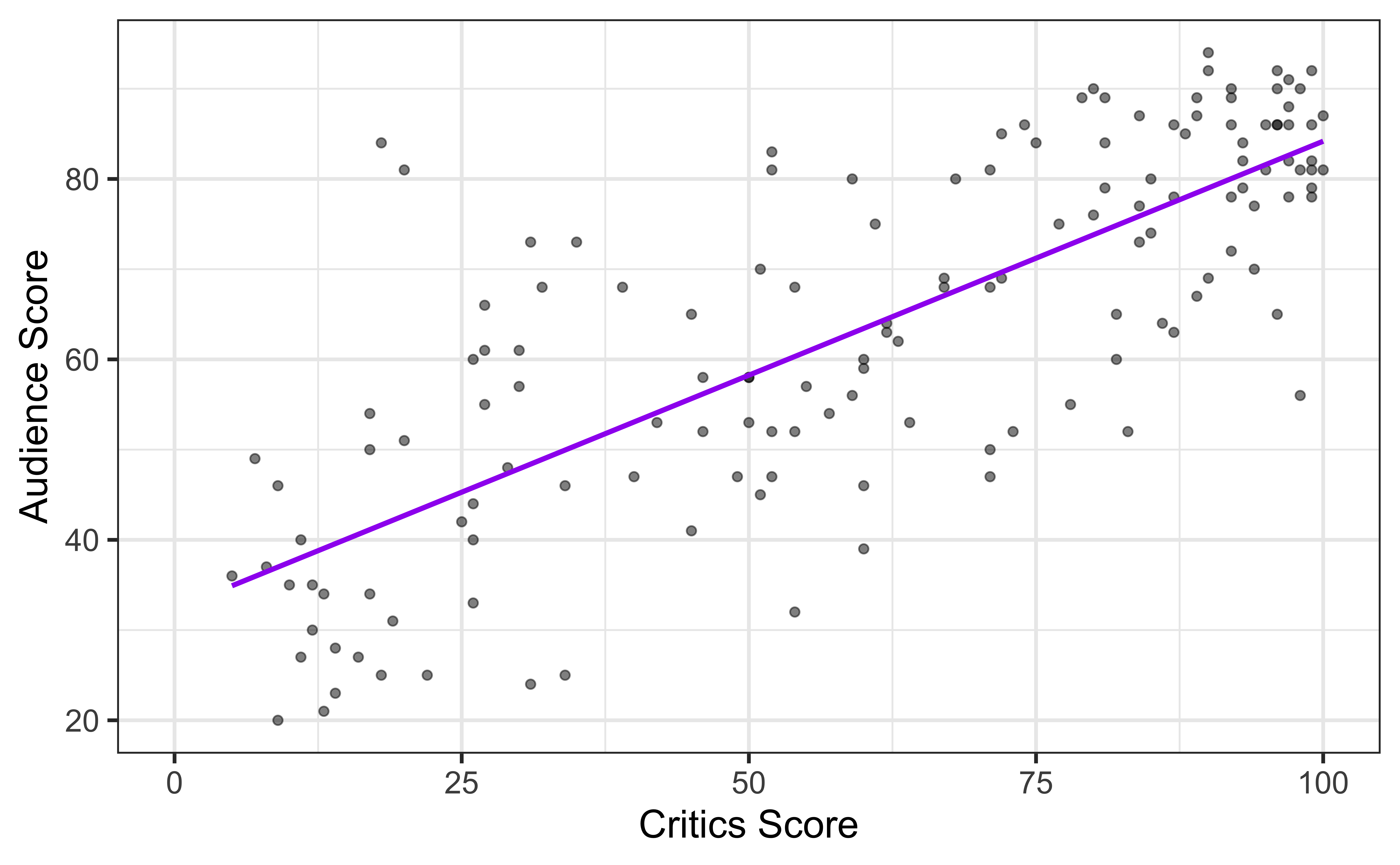
Suppose that a movie has a critics score of 0. According to this model, what is the movie’s predicted audience score?

Wrap up

Recap

  • Used simple linear regression to describe the relationship between a quantitative predictor and quantitative response variable.

  • Used the least squares method to estimate the slope and intercept.

  • We interpreted the slope and intercept.

    • Slope: For every one unit increase in \(x\), we expect y to change by \(\hat{\beta}_1\) units, on average.
    • Intercept: If \(x\) is 0, then we expect \(y\) to be \(\hat{\beta}_0\) units
  • Predicted the response given a value of the predictor variable.

  • Defined extrapolation and why we should avoid it.

Next class

We will talk about fitting linear models in R with tidymodels.