03:00
Simple Linear Regression
Prof. Maria Tackett
Aug 31, 2022
Announcements
R Resources page updated on the course website
Upcoming R workshops by Duke Center for Data and Visualization Sciences:
R for data science: getting started, EDA, data wrangling - Thu, Sep 15 at 1pm
R for data science: visualization, pivot, join, regression - Thu, Sep 22 at 1pm
Policyon requesting class recordings
See Week 01 for lecture notes, readings, AEs, and assignments
Meet your neighbor
Take a few moments to meet or (reconnect with) your neighbor!
- Name
- Year
- Major
- A highlight or something that stood out in the first two days of class

Data science life cycle from R for Data Science with modifications from The Art of Statistics: How to Learn from Data.
Topics
Use simple linear regression to describe the relationship between a quantitative predictor and quantitative response variable.
Estimate the slope and intercept of the regression line using the least squares method.
Interpret the slope and intercept of the regression line.
Predict the response given a value of the predictor variable.
Defined extrapolation and why we should avoid it.
Computation set up
# load packages
library(tidyverse)       # for data wrangling
library(tidymodels)      # for modeling
library(fivethirtyeight) # for the fandango dataset

# set default theme and larger font size for ggplot2
ggplot2::theme_set(ggplot2::theme_bw(base_size = 16))

# set default figure parameters for knitr
knitr::opts_chunk$set(
  fig.width = 8,
  fig.asp = 0.618,
  fig.retina = 3,
  dpi = 300,
  out.width = "80%"
)
Data
Movie ratings
- Data behind the FiveThirtyEight story Be Suspicious Of Online Movie Ratings, Especially Fandango’s
- In the fivethirtyeight package:
fandango - Contains every film that has at least 30 fan reviews on Fandango, an IMDb score, Rotten Tomatoes critic and user ratings, and Metacritic critic and user scores


Data prep
- Rename Rotten Tomatoes columns as
criticsandaudience - Rename the dataset as
movie_scores
Data overview
Rows: 146
Columns: 23
$ film                       <chr> "Avengers: Age of Ultron", "Cinderella", "A…
$ year                       <dbl> 2015, 2015, 2015, 2015, 2015, 2015, 2015, 2…
$ critics                    <int> 74, 85, 80, 18, 14, 63, 42, 86, 99, 89, 84,…
$ audience                   <int> 86, 80, 90, 84, 28, 62, 53, 64, 82, 87, 77,…
$ metacritic                 <int> 66, 67, 64, 22, 29, 50, 53, 81, 81, 80, 71,…
$ metacritic_user            <dbl> 7.1, 7.5, 8.1, 4.7, 3.4, 6.8, 7.6, 6.8, 8.8…
$ imdb                       <dbl> 7.8, 7.1, 7.8, 5.4, 5.1, 7.2, 6.9, 6.5, 7.4…
$ fandango_stars             <dbl> 5.0, 5.0, 5.0, 5.0, 3.5, 4.5, 4.0, 4.0, 4.5…
$ fandango_ratingvalue       <dbl> 4.5, 4.5, 4.5, 4.5, 3.0, 4.0, 3.5, 3.5, 4.0…
$ rt_norm                    <dbl> 3.70, 4.25, 4.00, 0.90, 0.70, 3.15, 2.10, 4…
$ rt_user_norm               <dbl> 4.30, 4.00, 4.50, 4.20, 1.40, 3.10, 2.65, 3…
$ metacritic_norm            <dbl> 3.30, 3.35, 3.20, 1.10, 1.45, 2.50, 2.65, 4…
$ metacritic_user_nom        <dbl> 3.55, 3.75, 4.05, 2.35, 1.70, 3.40, 3.80, 3…
$ imdb_norm                  <dbl> 3.90, 3.55, 3.90, 2.70, 2.55, 3.60, 3.45, 3…
$ rt_norm_round              <dbl> 3.5, 4.5, 4.0, 1.0, 0.5, 3.0, 2.0, 4.5, 5.0…
$ rt_user_norm_round         <dbl> 4.5, 4.0, 4.5, 4.0, 1.5, 3.0, 2.5, 3.0, 4.0…
$ metacritic_norm_round      <dbl> 3.5, 3.5, 3.0, 1.0, 1.5, 2.5, 2.5, 4.0, 4.0…
$ metacritic_user_norm_round <dbl> 3.5, 4.0, 4.0, 2.5, 1.5, 3.5, 4.0, 3.5, 4.5…
$ imdb_norm_round            <dbl> 4.0, 3.5, 4.0, 2.5, 2.5, 3.5, 3.5, 3.5, 3.5…
$ metacritic_user_vote_count <int> 1330, 249, 627, 31, 88, 34, 17, 124, 62, 54…
$ imdb_user_vote_count       <int> 271107, 65709, 103660, 3136, 19560, 39373, …
$ fandango_votes             <int> 14846, 12640, 12055, 1793, 1021, 397, 252, …
$ fandango_difference        <dbl> 0.5, 0.5, 0.5, 0.5, 0.5, 0.5, 0.5, 0.5, 0.5…
Movie ratings data
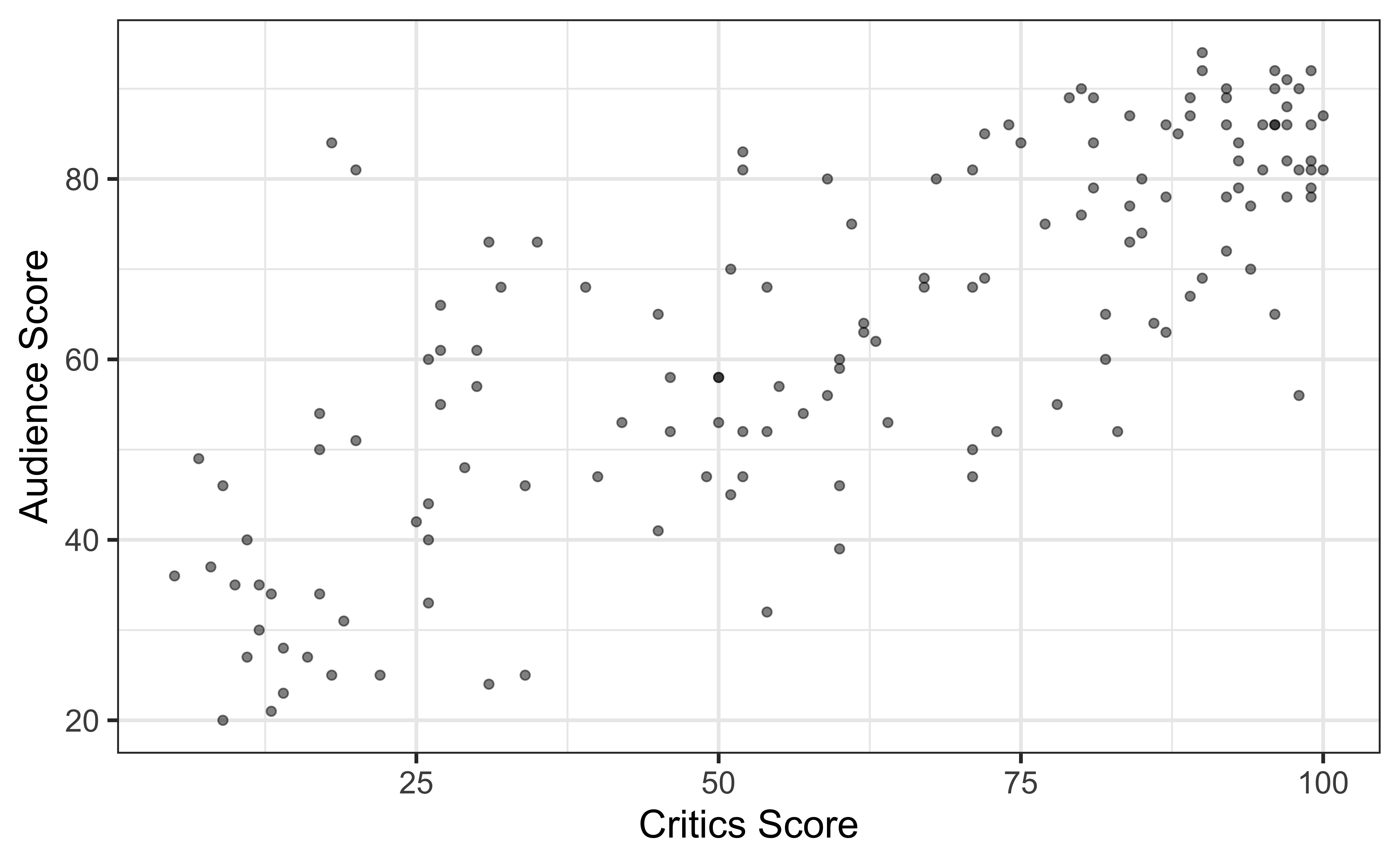
The data set contains the “Tomatometer” score (critics) and audience score (audience) for 146 movies rated on rottentomatoes.com.
Movie ratings data
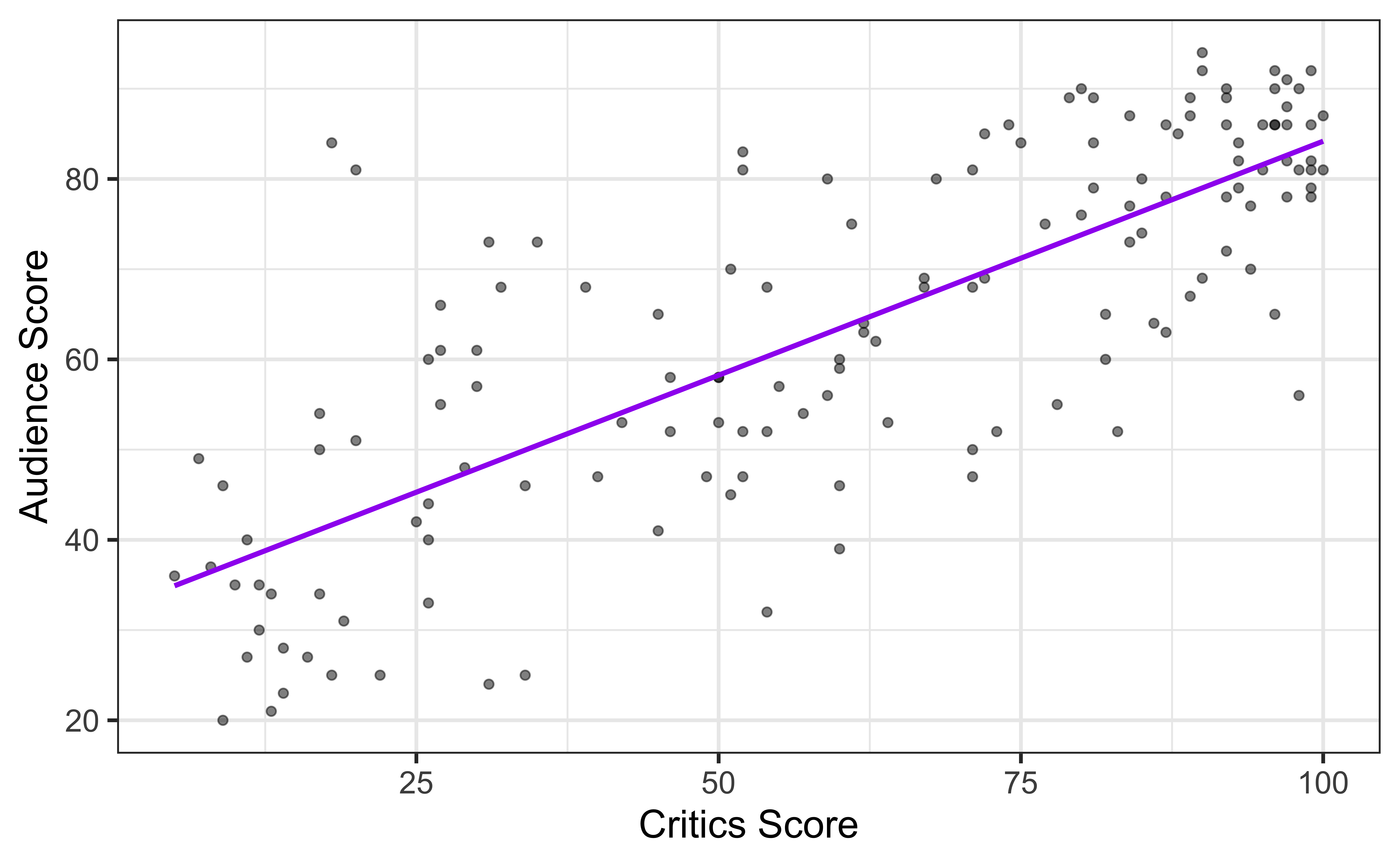
Goal: Fit a line to describe the relationship between the critics score and audience score.
Why fit a line?
We fit a line to accomplish one or both of the following:
Prediction
What is the audience score expected to be for an upcoming movie that received 35% from the critics?
Inference
Is the critics score a useful predictor of the audience score? By how much is the audience score expected to change for each additional point in the critics score?
Terminology
Response, Y: variable describing the outcome of interest
Predictor, X: variable we use to help understand the variability in the response

Regression model
A regression model is a function that describes the relationship between the response, \(Y\), and the predictor, \(X\).
\[\begin{aligned} Y &= \color{black}{\textbf{Model}} + \text{Error} \\[8pt] &= \color{black}{\mathbf{f(X)}} + \epsilon \\[8pt] &= \color{black}{\boldsymbol{\mu_{Y|X}}} + \epsilon \end{aligned}\]Regression model
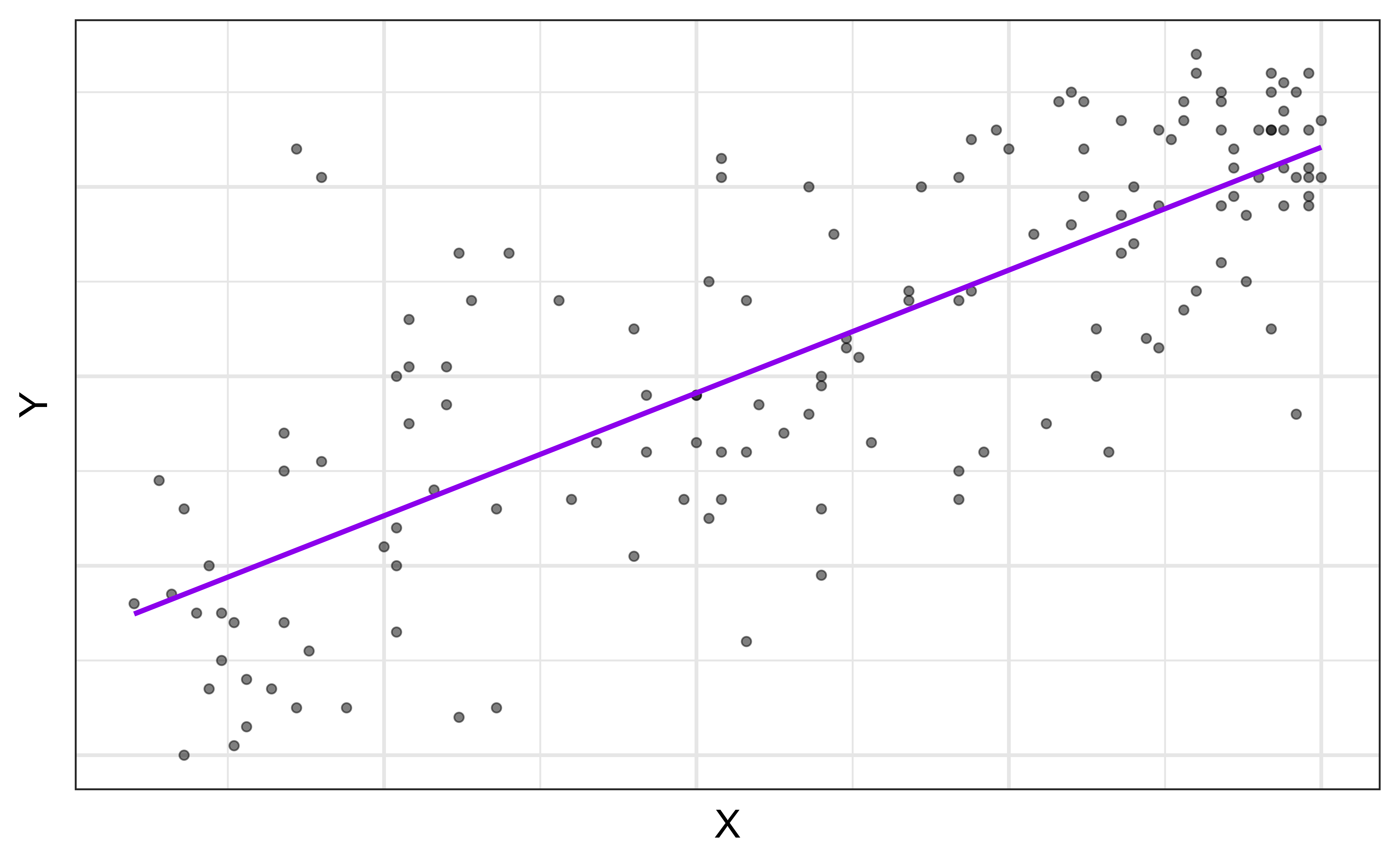
\(\mu_{Y|X}\) is the mean value of \(Y\) given a particular value of \(X\).
Regression model
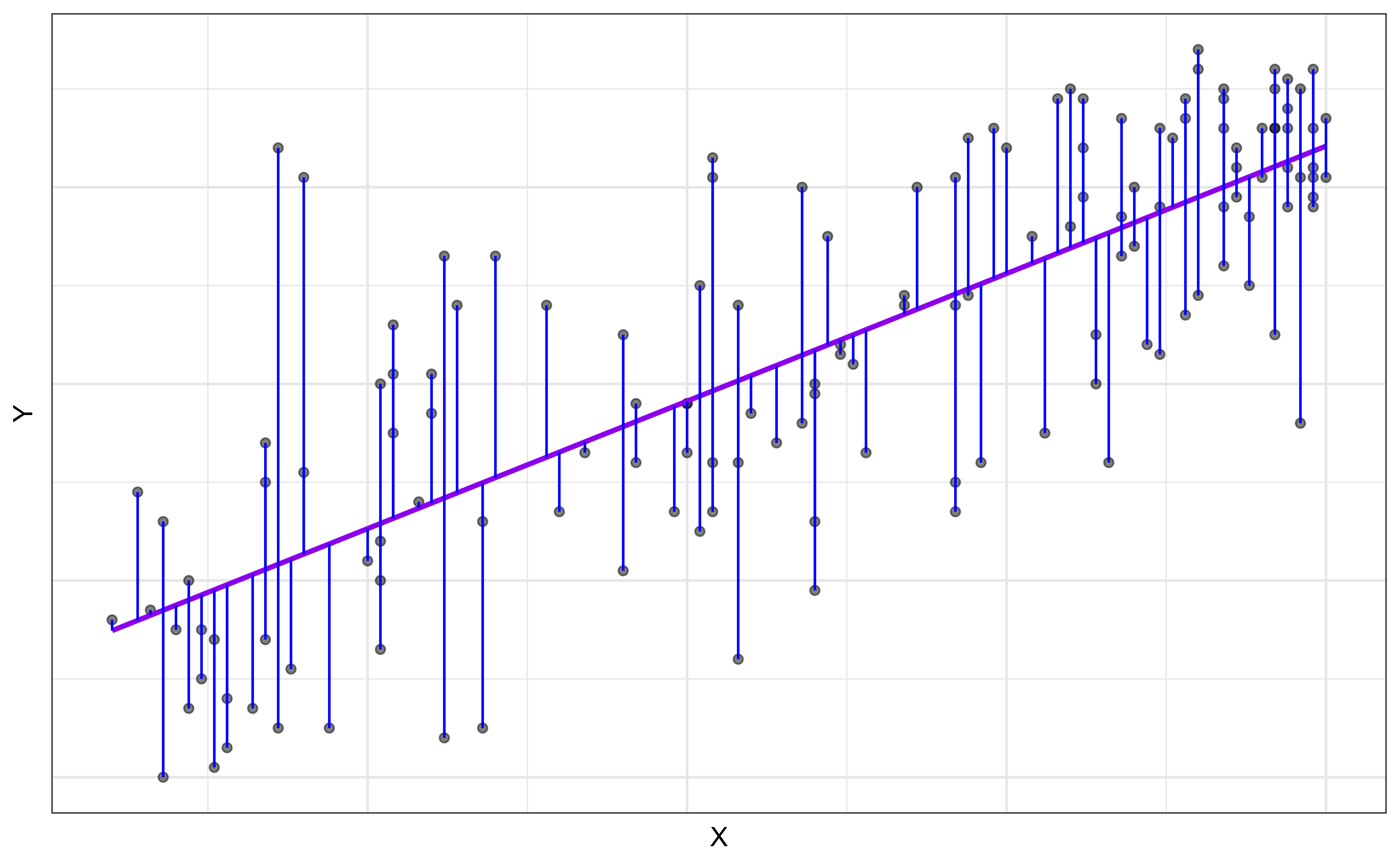
\[ \begin{aligned} Y &= \color{purple}{\textbf{Model}} + \color{blue}{\textbf{Error}} \\[5pt] &= \color{purple}{\mathbf{f(X)}} + \color{blue}{\boldsymbol{\epsilon}} \\[5pt] &= \color{purple}{\boldsymbol{\mu_{Y|X}}} + \color{blue}{\boldsymbol{\epsilon}} \\[5pt] \end{aligned} \]
Simple linear regression
Simple linear regression
When we have a quantitative response, \(Y\), and a single quantitative predictor, \(X\), we can use a simple linear regression model to describe the relationship between \(Y\) and \(X\). \[\Large{Y = \mathbf{\beta_0 + \beta_1 X} + \epsilon}\]
- \(\beta_1\): True slope of the relationship between \(X\) and \(Y\)
- \(\beta_0\): True intercept of the relationship between \(X\) and \(Y\)
- \(\epsilon\): Error
Simple linear regression
\[\Large{\hat{Y} = \hat{\beta}_0 + \hat{\beta}_1 X}\]
- \(\hat{\beta}_1\): Estimated slope of the relationship between \(X\) and \(Y\)
- \(\hat{\beta}_0\): Estimated intercept of the relationship between \(X\) and \(Y\)
- No error term!
Choosing values for \(\hat{\beta}_1\) and \(\hat{\beta}_0\)
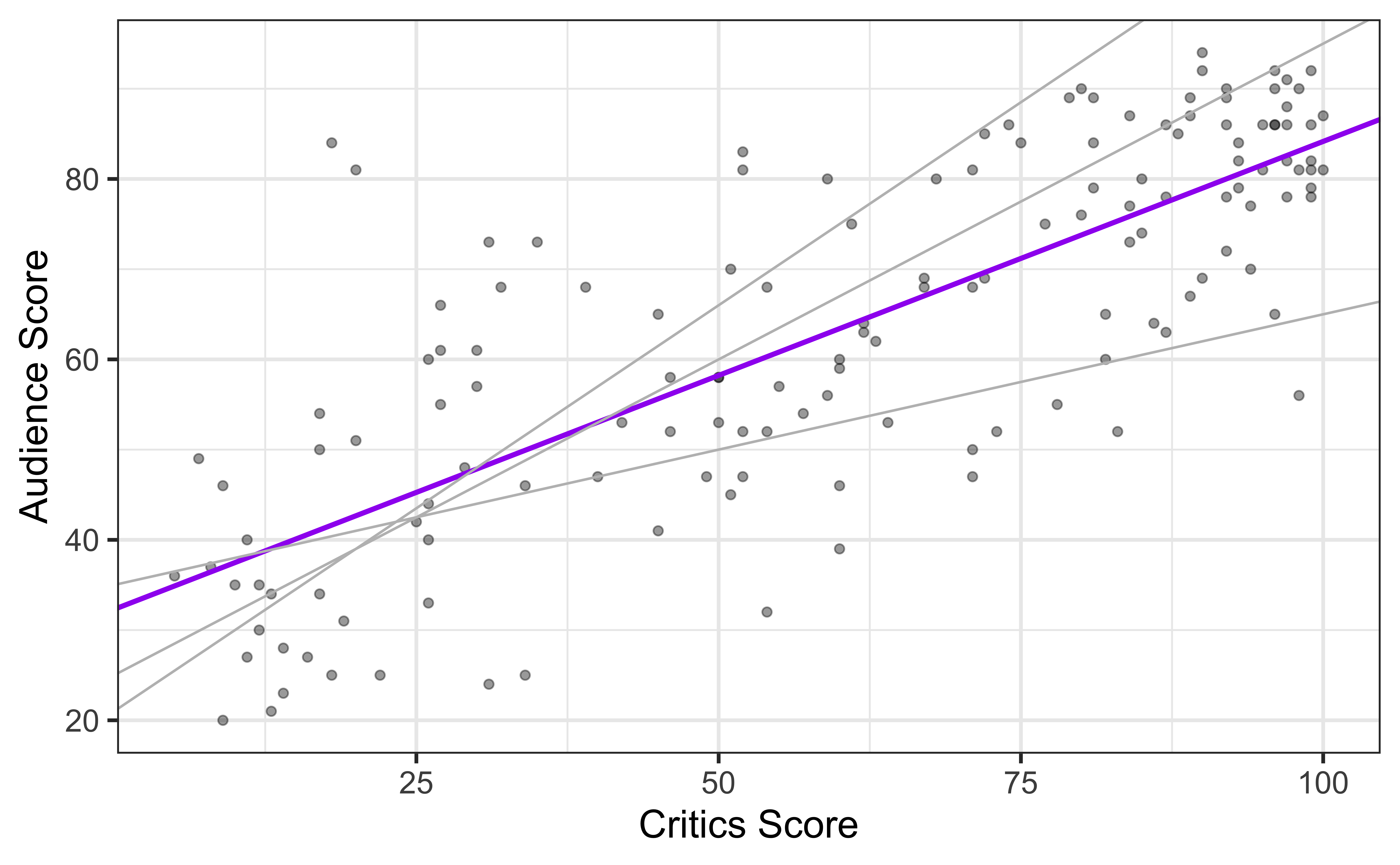
Residuals
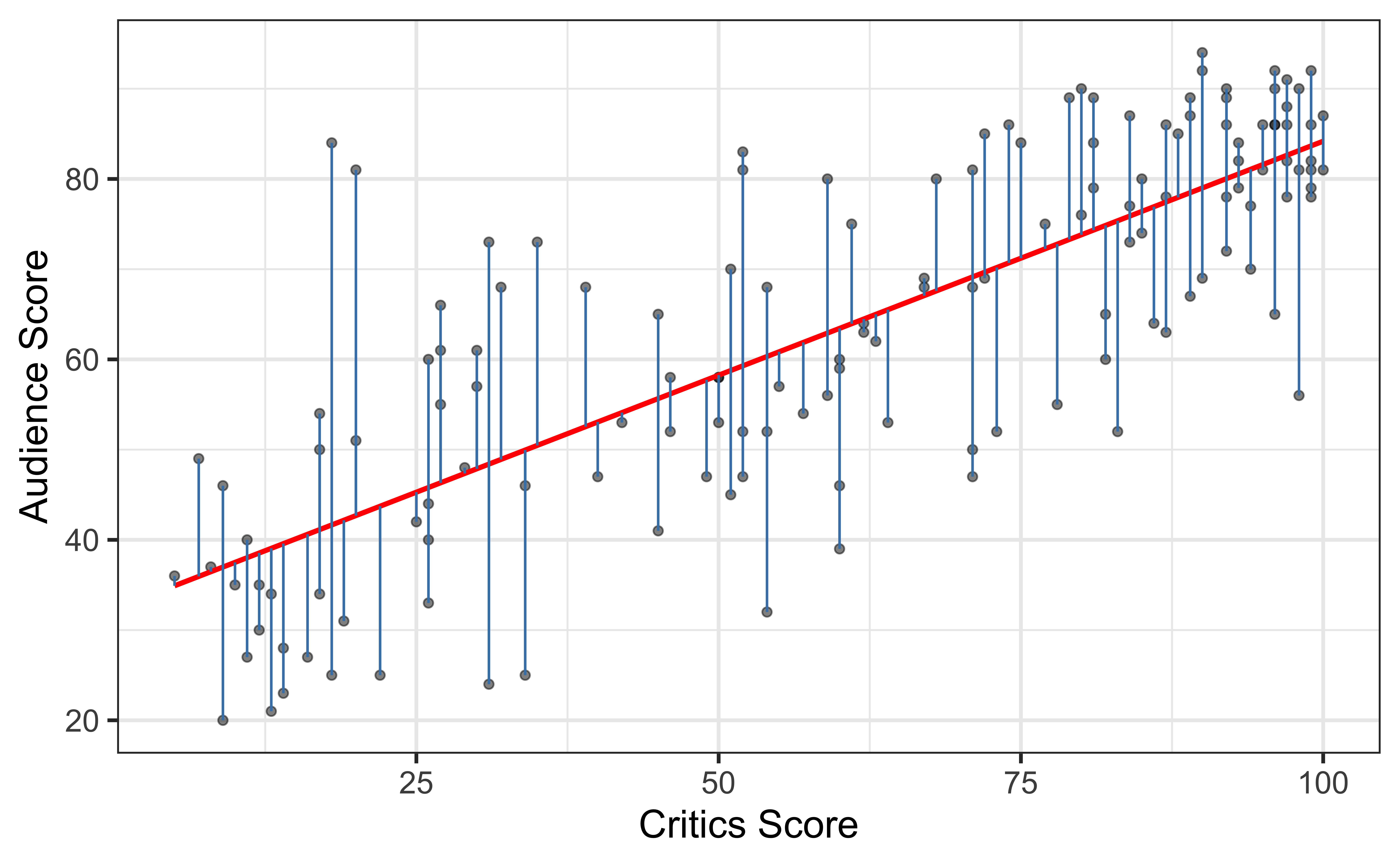
\[\text{residual} = \text{observed} - \text{predicted} = y - \hat{y}\]
Least squares line
- The residual for the \(i^{th}\) observation is
\[e_i = \text{observed} - \text{predicted} = y_i - \hat{y}_i\]
- The sum of squared residuals is
\[e^2_1 + e^2_2 + \dots + e^2_n\]
- The least squares line is the one that minimizes the sum of squared residuals
Slope and intercept
Properties of least squares regression
The regression line goes through the center of mass point, the coordinates corresponding to average \(X\) and average \(Y\): \(\hat{\beta}_0 = \bar{Y} - \hat{\beta}_1\bar{X}\)
The slope has the same sign as the correlation coefficient: \(\hat{\beta}_1 = r \frac{s_Y}{s_X}\)
The sum of the residuals is zero: \(\sum_{i = 1}^n \epsilon_i = 0\)
The residuals and \(X\) values are uncorrelated
Estimating the slope
\[\large{\hat{\beta}_1 = r \frac{s_Y}{s_X}}\]
Click here for details on deriving the equations for slope and intercept.
Estimating the intercept
\[\large{\hat{\beta}_0 = \bar{Y} - \hat{\beta}_1\bar{X}}\]
Click here for details on deriving the equations for slope and intercept.
Interpretation
Post your answers to the following questions on Ed Discussion:
The slope of the model for predicting audience score from critics score is 0.5187 . Which of the following is the best interpretation of this value?
32.3142 is the predicted mean audience score for what type of movies?
Link for Section 001 (10:15am lecture)
Link for Section 002 (3:30pm lecture)
03:00
Does it make sense to interpret the intercept?
✅ The intercept is meaningful in the context of the data if
the predictor can feasibly take values equal to or near zero, or
there are values near zero in the observed data.
🛑 Otherwise, the intercept may not be meaningful!
Prediction
Making a prediction
Suppose that a movie has a critics score of 70. According to this model, what is the movie’s predicted audience score?
\[\begin{aligned} \widehat{\text{audience}} &= 32.3142 + 0.5187 \times \text{critics} \\ &= 32.3142 + 0.5187 \times 70 \\ &= 68.6232 \end{aligned}\]⚠️ Extrapolation
Using the model to predict for values outside the range of the original data is extrapolation.
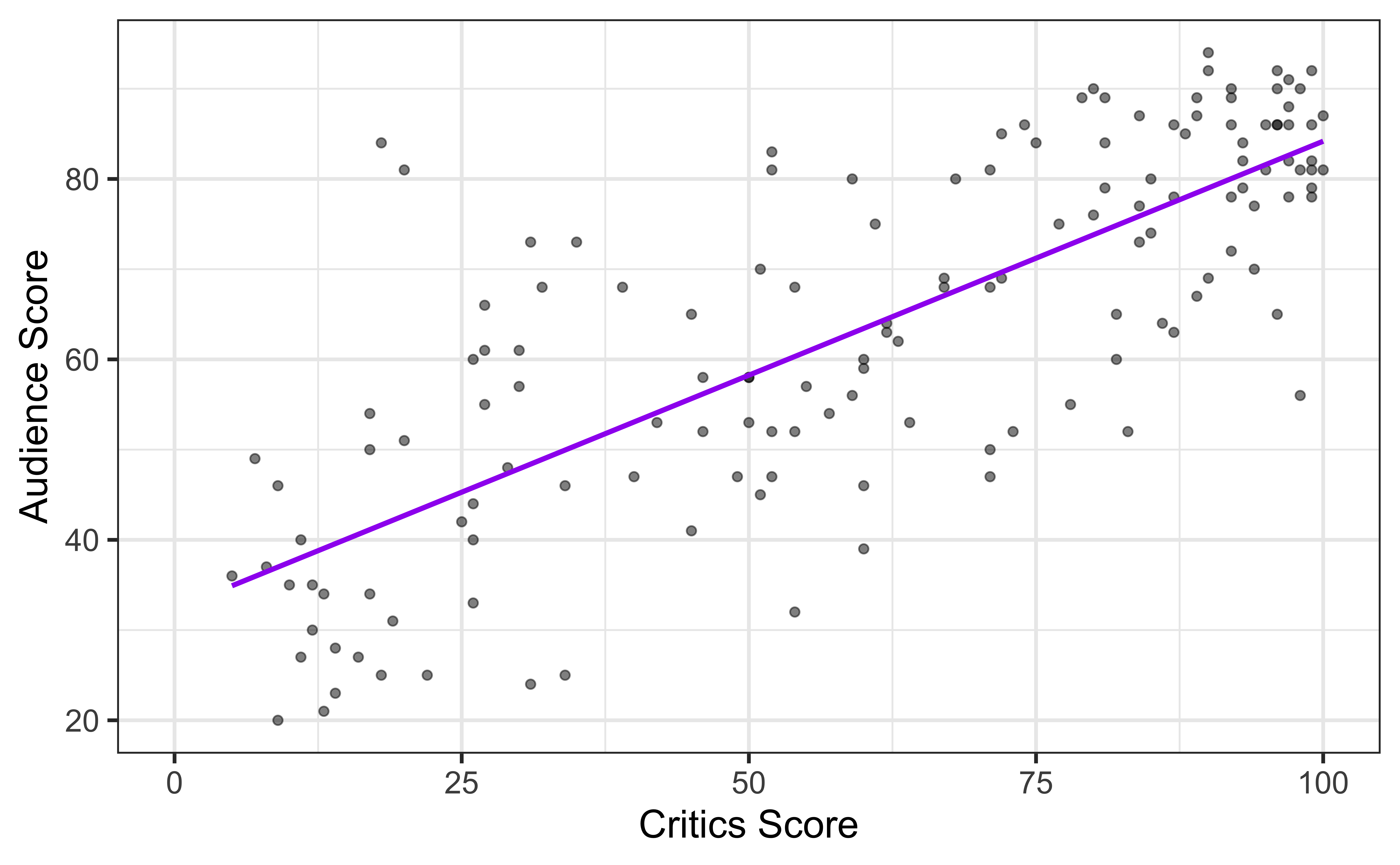
Suppose that a movie has a critics score of 0. According to this model, what is the movie’s predicted audience score?
Wrap up
Recap
Used simple linear regression to describe the relationship between a quantitative predictor and quantitative response variable.
Used the least squares method to estimate the slope and intercept.
We interpreted the slope and intercept.
- Slope: For every one unit increase in \(x\), we expect y to change by \(\hat{\beta}_1\) units, on average.
- Intercept: If \(x\) is 0, then we expect \(y\) to be \(\hat{\beta}_0\) units
Predicted the response given a value of the predictor variable.
Defined extrapolation and why we should avoid it.
Next class
We will talk about fitting linear models in R with tidymodels.
Reserve STA 210 Docker Container before Monday’s lecture
Complete the STA 210 Student Survey (will ask for a GitHub username) by Friday at 11:59pm
