SLR: Conditions

Prof. Maria Tackett

Sep 21, 2022

Announcements

  • HW 01: due TODAY at 11:59pm

  • Statistics experience - due Fri, Dec 09 at 11:59pm

  • Aaditya’s office hours today: 1 - 2pm and 7 -8pm on Zoom (link in Sakai)

  • See Week 04 for this week’s activities.

  • Updated masking policy starting Sep 22

  • Looking ahead: Exam 01: Sep 28 - 30

Exam 01

  • Released Sep 28 late afternoon, due Sep 30 at 11:59pm.

    • No labs or office hours Sep 28 - 30
  • Covers content Weeks 01 - 05

  • Conceptual questions + analysis problems

  • Will receive exam through GitHub repo, use a reproducible workflow and submit on GitHub and Gradescope (like labs and HW)

  • Lecture recordings for Weeks 01 -05 available here until September 28 at 11:59pm.

  • Lab and HW solutions will be posted after the late submission deadlines.

  • Exam 01 review in class on September 28

Computational set up

# load packages
library(tidyverse)   # for data wrangling and visualization
library(tidymodels)  # for modeling
library(openintro)   # for the duke_forest dataset
library(scales)      # for pretty axis labels
library(knitr)       # for pretty tables
library(kableExtra)  # also for pretty tables
library(patchwork)   # arrange plots

# set default theme and larger font size for ggplot2
ggplot2::theme_set(ggplot2::theme_bw(base_size = 20))

Regression model, revisited

df_fit <- linear_reg() |>
  set_engine("lm") |>
  fit(price ~ area, data = duke_forest)

tidy(df_fit) |>
  kable(digits = 3)
term estimate std.error statistic p.value
(Intercept) 116652.325 53302.463 2.188 0.031
area 159.483 18.171 8.777 0.000

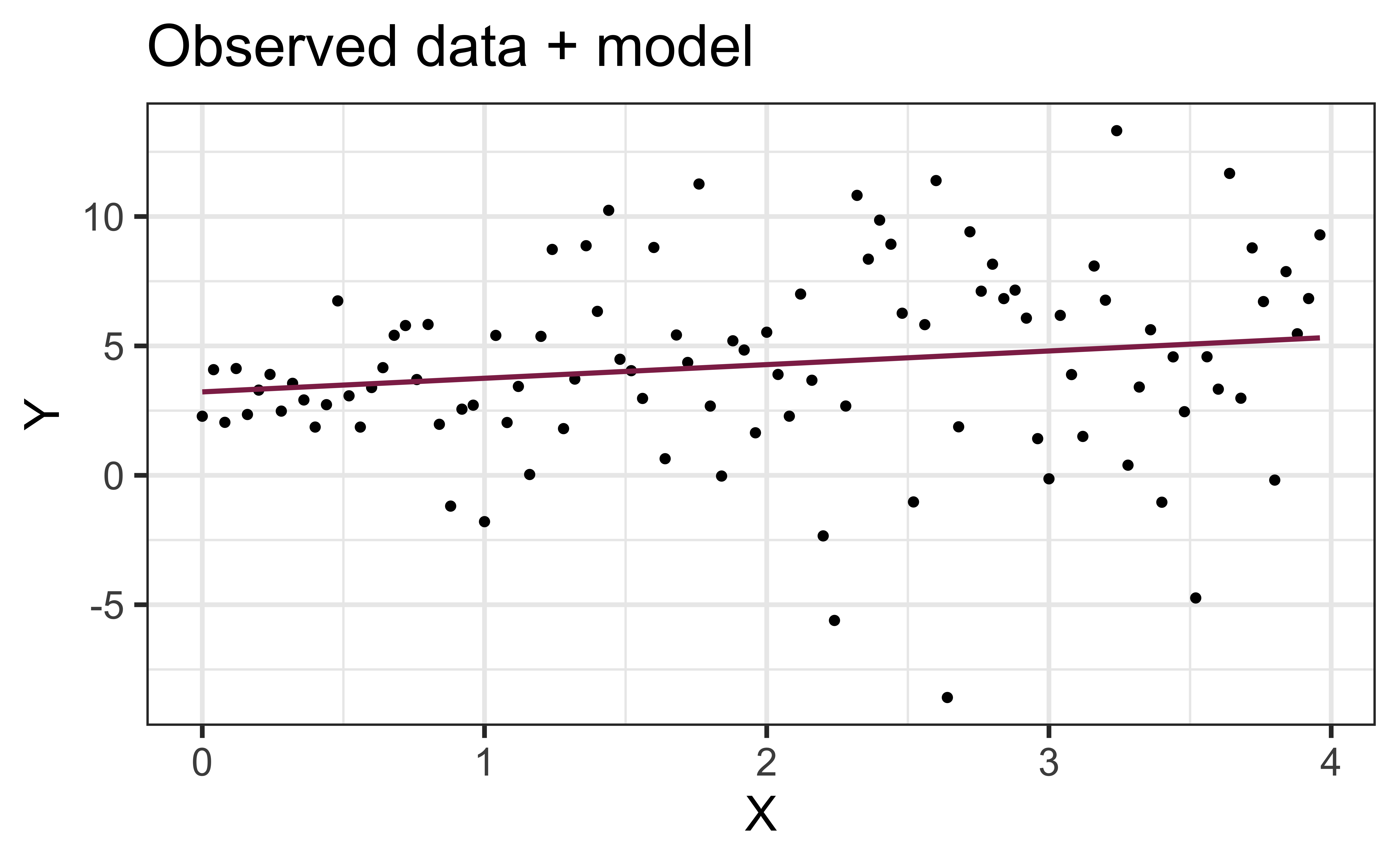
Mathematical representation, visualized

\[ Y|X \sim N(\beta_0 + \beta_1 X, \sigma_\epsilon^2) \]
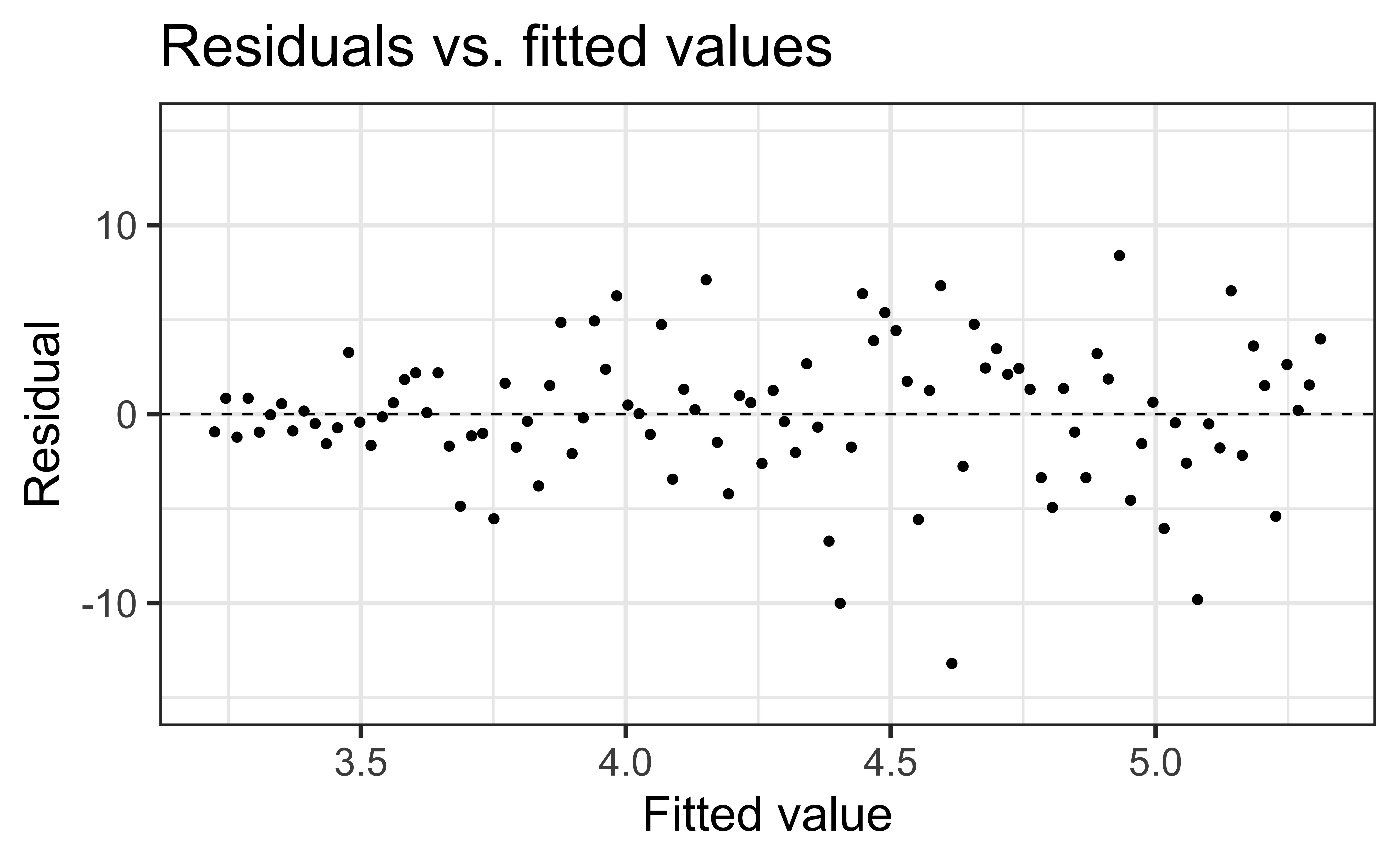
Model conditions

  1. Linearity: There is a linear relationship between the outcome and predictor variables
  2. Constant variance: The variability of the errors is equal for all values of the predictor variable, i.e. the errors are homeoscedastic
  3. Normality: The errors follow a normal distribution
  4. Independence: The errors are independent from each other

Linearity

✅ The residuals vs. fitted values plot should show a random scatter of residuals (no distinguishable pattern or structure)

Residuals vs. fitted values (code)

df_aug <- augment(df_fit$fit)

ggplot(df_aug, aes(x = .fitted, y = .resid)) +
  geom_point() +
  geom_hline(yintercept = 0, linetype = "dashed") +
  ylim(-1000000, 1000000) +
  labs(
    x = "Fitted value", y = "Residual",
    title = "Residuals vs. fitted values"
  )

Non-linear relationships

Constant variance

✅ The vertical spread of the residuals should be relatively constant across the plot

Non-constant variance
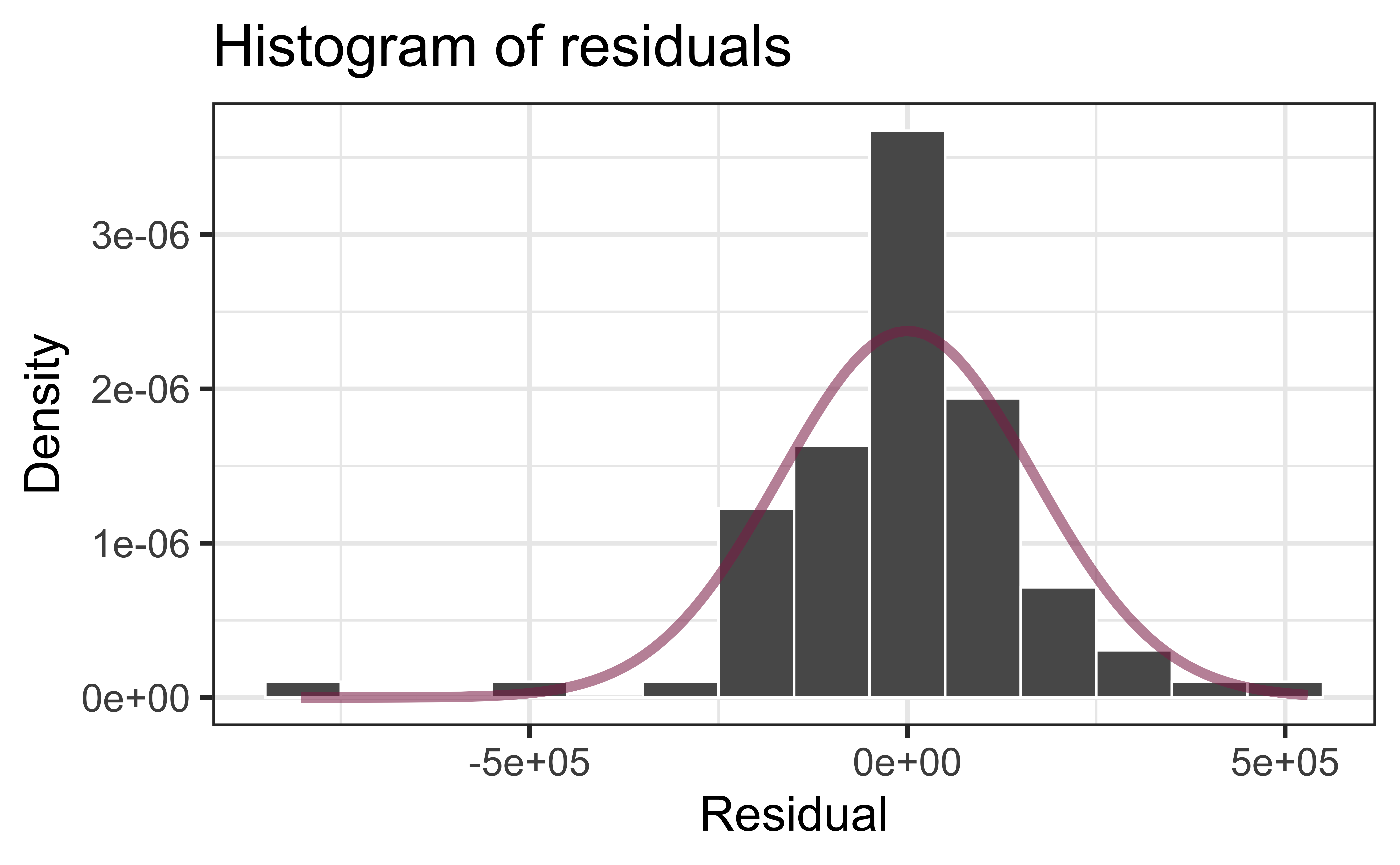
Normality

Independence

  • We can often check the independence assumption based on the context of the data and how the observations were collected

  • If the data were collected in a particular order, examine a scatterplot of the residuals versus order in which the data were collected

✅ If this is a random sample of Duke Houses, the error for one house does not tell us anything about the error for another use

Recap

Used residual plots to check conditions for SLR:

  • Linearity
  • Constant variance
  • Normality
  • Independence

Which of these conditions are required for fitting a SLR? Which for simulation-based inference for the slope for an SLR? Which for inference with mathematical models?

03:00