Feature engineering

Prof. Maria Tackett

Oct 03, 2022

Announcements

Click here for slides from presentation about the Academic Resource Center.

Topics

• Understanding categorical predictors and interaction terms

• Feature engineering

Computational setup

# load packages
library(tidyverse)
library(tidymodels)
library(openintro)
library(patchwork)
library(knitr)
library(kableExtra)
library(colorblindr)

# set default theme and larger font size for ggplot2
ggplot2::theme_set(ggplot2::theme_bw(base_size = 20))

Types of predictors

Data: Peer-to-peer lender

Today’s data is a sample of 50 loans made through a peer-to-peer lending club. The data is in the loan50 data frame in the openintro R package.

# A tibble: 50 × 4
   annual_income debt_to_income verified_income interest_rate
           <dbl>          <dbl> <fct>                   <dbl>
 1         59000         0.558  Not Verified            10.9 
 2         60000         1.31   Not Verified             9.92
 3         75000         1.06   Verified                26.3 
 4         75000         0.574  Not Verified             9.92
 5        254000         0.238  Not Verified             9.43
 6         67000         1.08   Source Verified          9.92
 7         28800         0.0997 Source Verified         17.1 
 8         80000         0.351  Not Verified             6.08
 9         34000         0.698  Not Verified             7.97
10         80000         0.167  Source Verified         12.6 
# … with 40 more rows

Variables

Predictors:

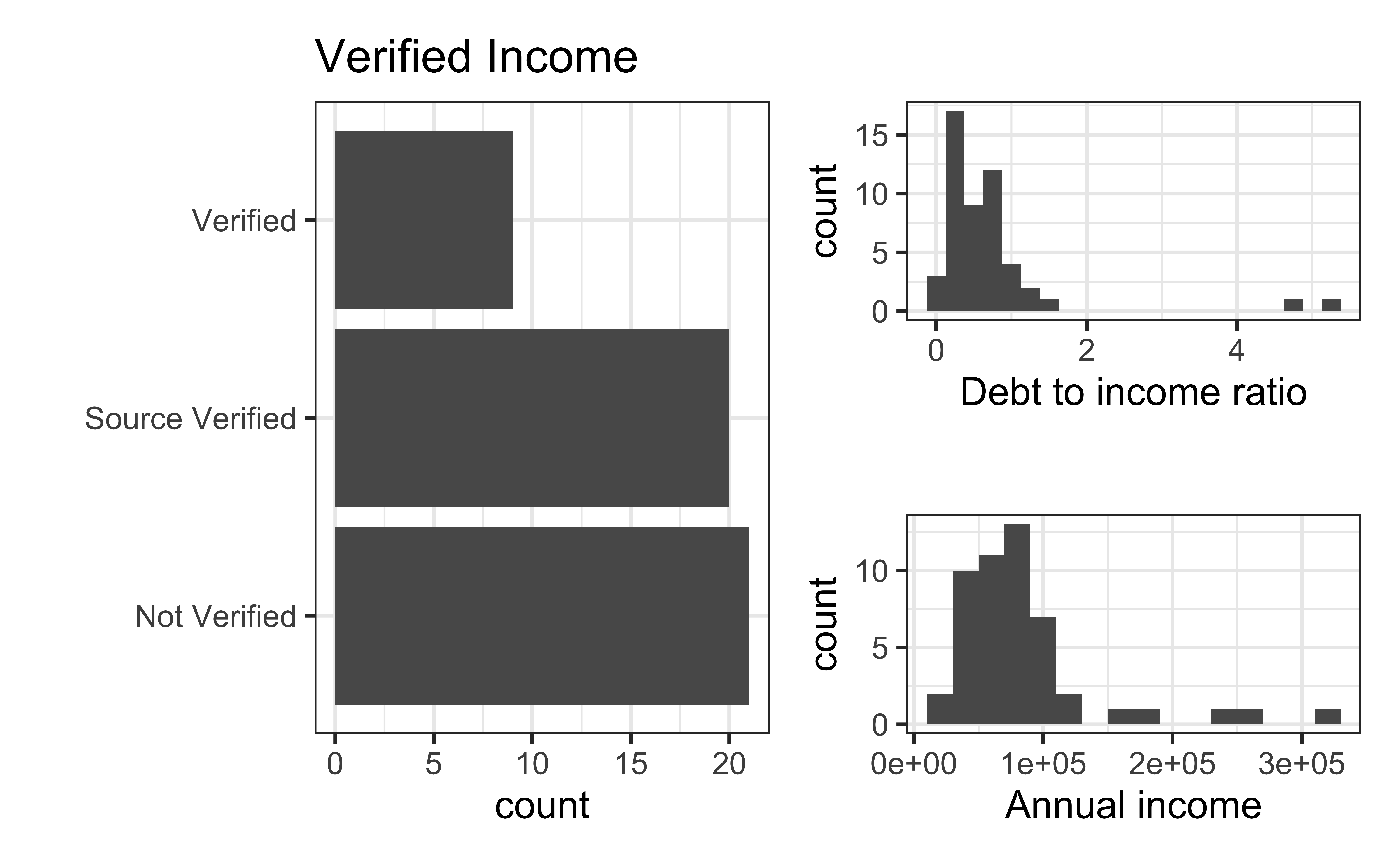
• annual_income: Annual income
• debt_to_income: Debt-to-income ratio, i.e. the percentage of a borrower’s total debt divided by their total income
• verified_income: Whether borrower’s income source and amount have been verified (Not Verified, Source Verified, Verified)

Outcome: interest_rate: Interest rate for the loan

Outcome: interest_rate

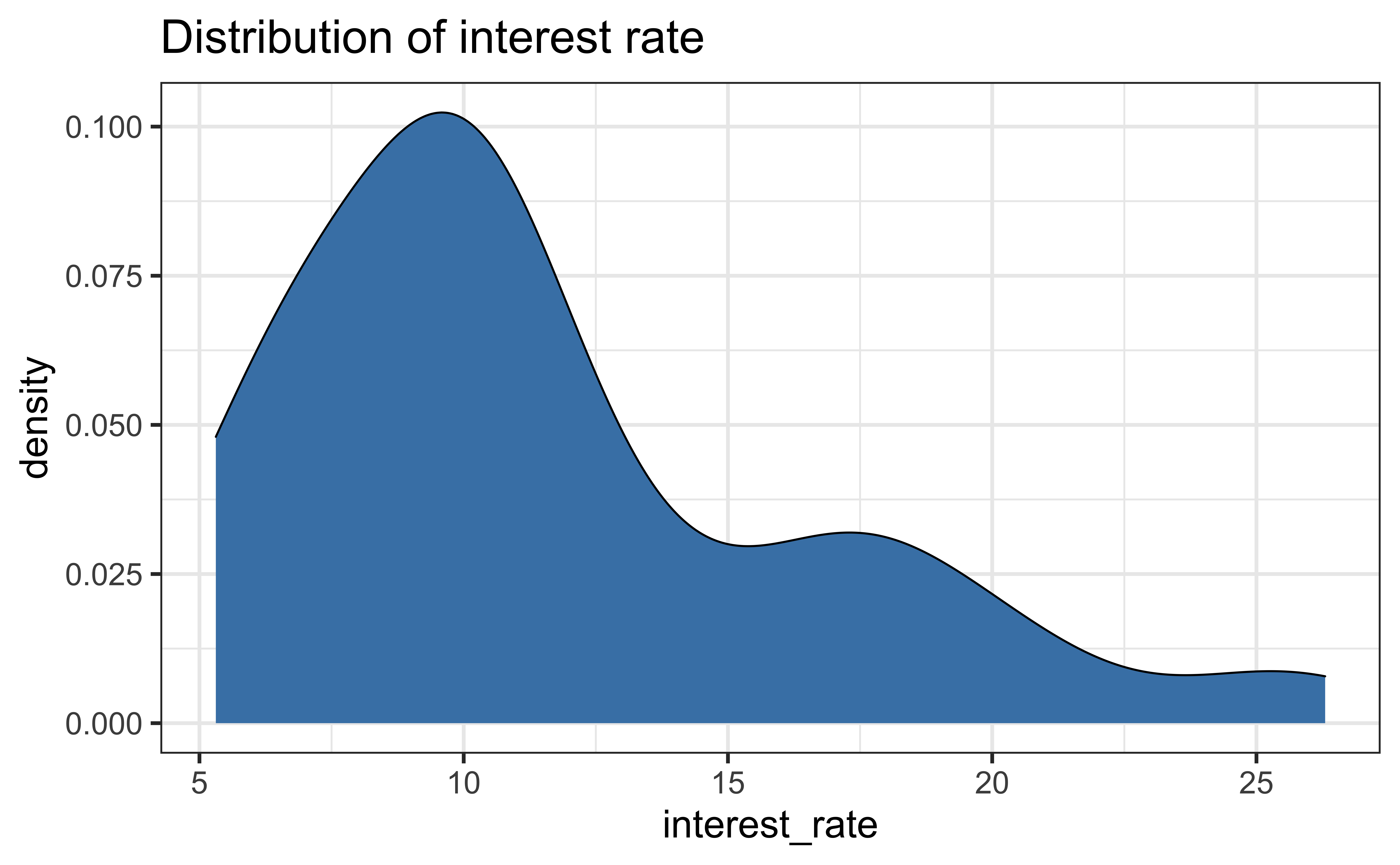
min	median	max	iqr
5.31	9.93	26.3	5.755

Predictors

Data manipulation 1: Rescale income

loan50 <- loan50 |>
  mutate(annual_income_th = annual_income / 1000)

ggplot(loan50, aes(x = annual_income_th)) +
  geom_histogram(binwidth = 20) +
  labs(title = "Annual income (in $1000s)", 
       x = "")

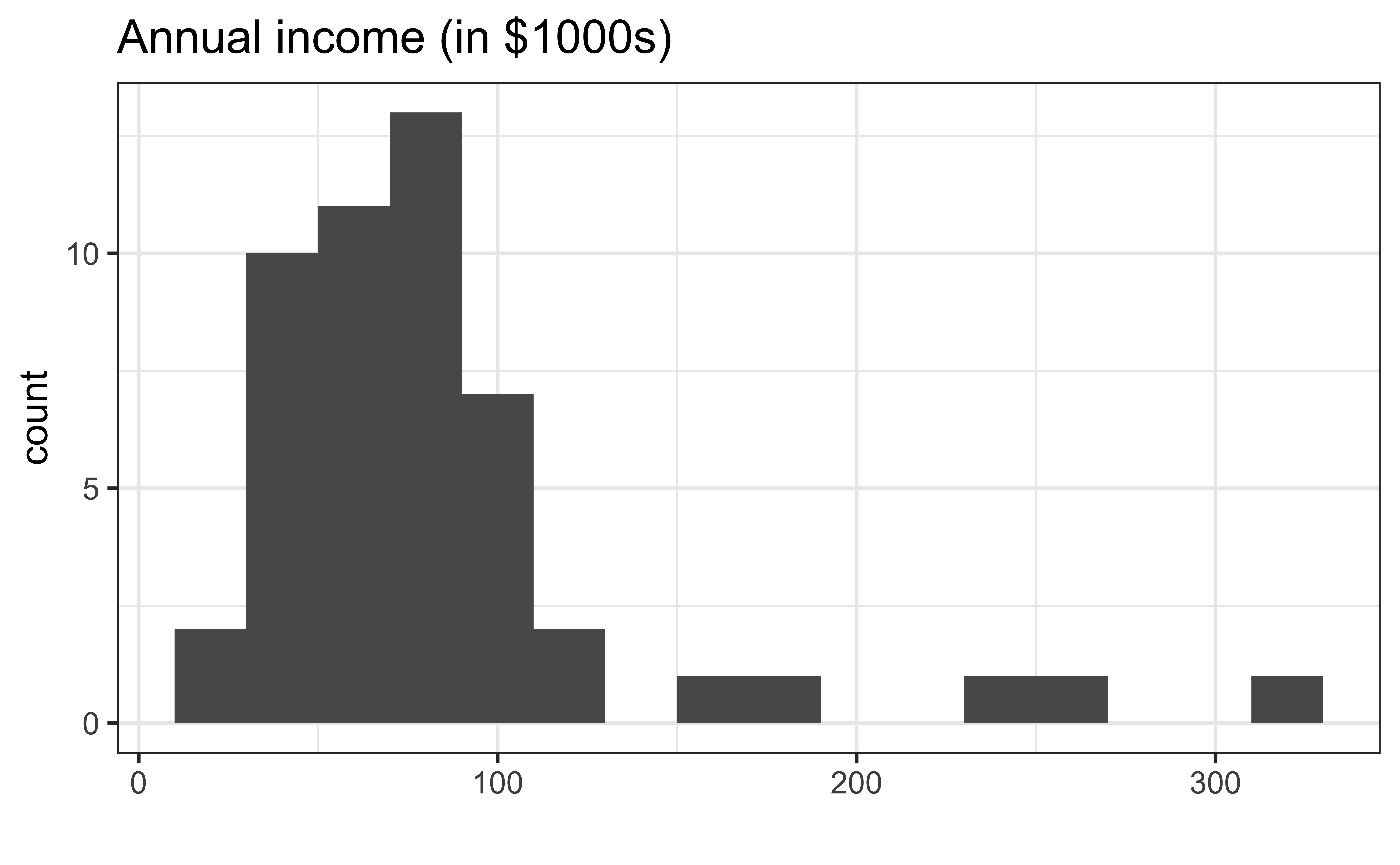
Data manipulation 2: Mean-center numeric predictors

loan50 <- loan50 |>
  mutate(
    debt_inc_cent = debt_to_income - mean(debt_to_income), 
    annual_income_th_cent = annual_income_th - mean(annual_income_th)
    )

Data manipulation 3: Create indicator variables for verified_income

loan50 <- loan50 |>
  mutate(
    not_verified = if_else(verified_income == "Not Verified", 1, 0),
    source_verified = if_else(verified_income == "Source Verified", 1, 0),
    verified = if_else(verified_income == "Verified", 1, 0)
  )

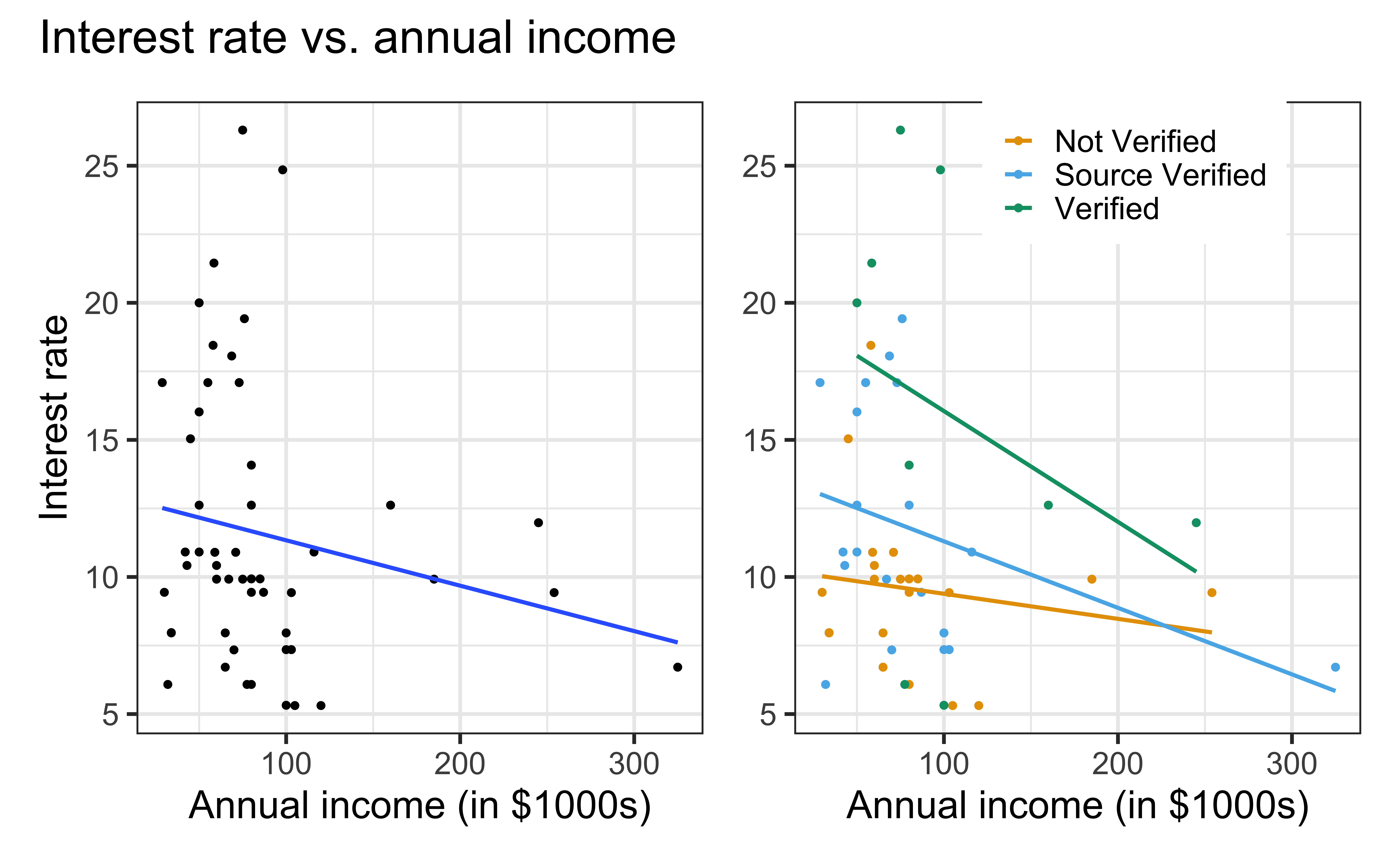
Interest rate vs. annual income

The lines are not parallel indicating there is an interaction effect. The slope of annual income differs based on the income verification.

Data manipulation 4: Create interaction variables

Defining the interaction variable in the model formula as verified_income * annual_income_th_cent is an implicit data manipulation step as well

Rows: 50
Columns: 9
$ `(Intercept)`                                          <dbl> 1, 1, 1, 1, 1, …
$ debt_inc_cent                                          <dbl> -0.16511719, 0.…
$ annual_income_th_cent                                  <dbl> -27.17, -26.17,…
$ `verified_incomeNot Verified`                          <dbl> 1, 1, 0, 1, 1, …
$ `verified_incomeSource Verified`                       <dbl> 0, 0, 0, 0, 0, …
$ verified_incomeVerified                                <dbl> 0, 0, 1, 0, 0, …
$ `annual_income_th_cent:verified_incomeNot Verified`    <dbl> -27.17, -26.17,…
$ `annual_income_th_cent:verified_incomeSource Verified` <dbl> 0.00, 0.00, 0.0…
$ `annual_income_th_cent:verified_incomeVerified`        <dbl> 0.00, 0.00, -11…

Interaction term in the model

int_cent_int_fit <- linear_reg() |>
  set_engine("lm") |>
  fit(interest_rate ~ debt_inc_cent  +  verified_income + 
        annual_income_th_cent + verified_income * annual_income_th_cent,
      data = loan50)

term	estimate	std.error	statistic	p.value
(Intercept)	9.484	0.989	9.586	0.000
debt_inc_cent	0.691	0.685	1.009	0.319
verified_incomeSource Verified	2.157	1.418	1.522	0.135
verified_incomeVerified	7.181	1.870	3.840	0.000
annual_income_th_cent	-0.007	0.020	-0.341	0.735
verified_incomeSource Verified:annual_income_th_cent	-0.016	0.026	-0.643	0.523
verified_incomeVerified:annual_income_th_cent	-0.032	0.033	-0.979	0.333

Interpreting interaction terms

• What the interaction means: The effect of annual income on the interest rate differs by -0.016 when the income is source verified compared to when it is not verified, holding all else constant.
• Interpreting annual_income for source verified: If the income is source verified, we expect the interest rate to decrease by 0.023% (-0.007 + -0.016) for each additional thousand dollars in annual income, holding all else constant.

Understanding the model

\[ \begin{aligned} \hat{interest\_rate} &= 9.484 + 0.691 \times debt\_inc\_cent\\ &- 0.007 \times annual\_income\_th\_cent \\ &+ 2.157 \times SourceVerified + 7.181 \times Verified \\ &- 0.016 \times annual\_inc\_th\_cent \times SourceVerified\\ &- 0.032 \times annual\_inc\_th\_cent \times Verified \end{aligned} \]

1. What is \(p\), the number of predictor terms in the model?
2. Write the equation of the model to predict interest rate for applicants with Not Verified income.
3. Write the equation of the model to predict interest rate for applicants with Verified income.

Feature engineering

Topics

• Review: Training and testing splits
• Feature engineering with recipes

Computational setup

# load packages
library(tidyverse)
library(tidymodels)
library(gghighlight)
library(knitr)

# set default theme and larger font size for ggplot2
ggplot2::theme_set(ggplot2::theme_minimal(base_size = 20))

Introduction

The Office

Data

The data come from data.world, by way of TidyTuesday

office_ratings <- read_csv("data/office_ratings.csv")
office_ratings

# A tibble: 188 × 6
   season episode title             imdb_rating total_votes air_date  
    <dbl>   <dbl> <chr>                   <dbl>       <dbl> <date>    
 1      1       1 Pilot                     7.6        3706 2005-03-24
 2      1       2 Diversity Day             8.3        3566 2005-03-29
 3      1       3 Health Care               7.9        2983 2005-04-05
 4      1       4 The Alliance              8.1        2886 2005-04-12
 5      1       5 Basketball                8.4        3179 2005-04-19
 6      1       6 Hot Girl                  7.8        2852 2005-04-26
 7      2       1 The Dundies               8.7        3213 2005-09-20
 8      2       2 Sexual Harassment         8.2        2736 2005-09-27
 9      2       3 Office Olympics           8.4        2742 2005-10-04
10      2       4 The Fire                  8.4        2713 2005-10-11
# … with 178 more rows

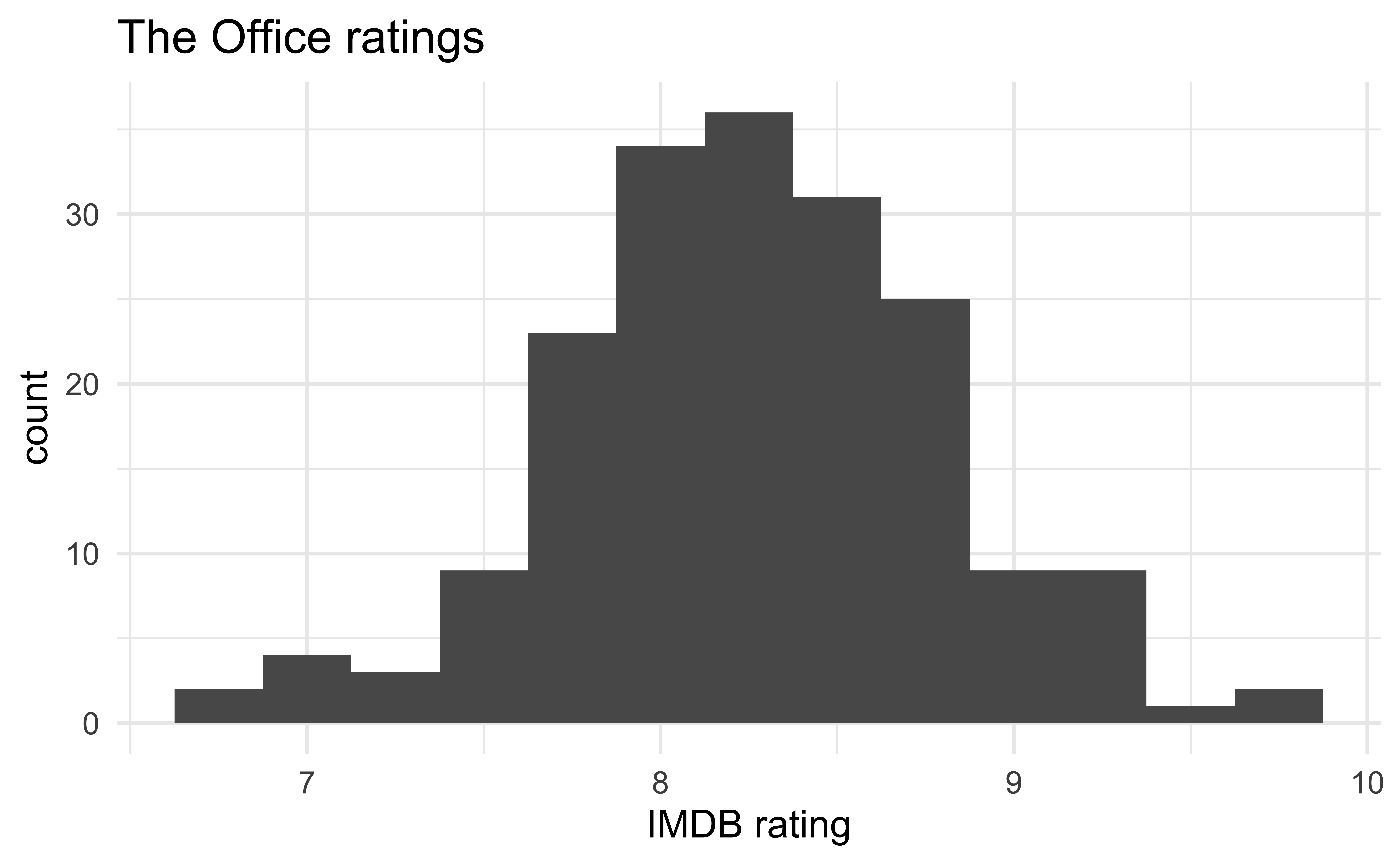
IMDB ratings

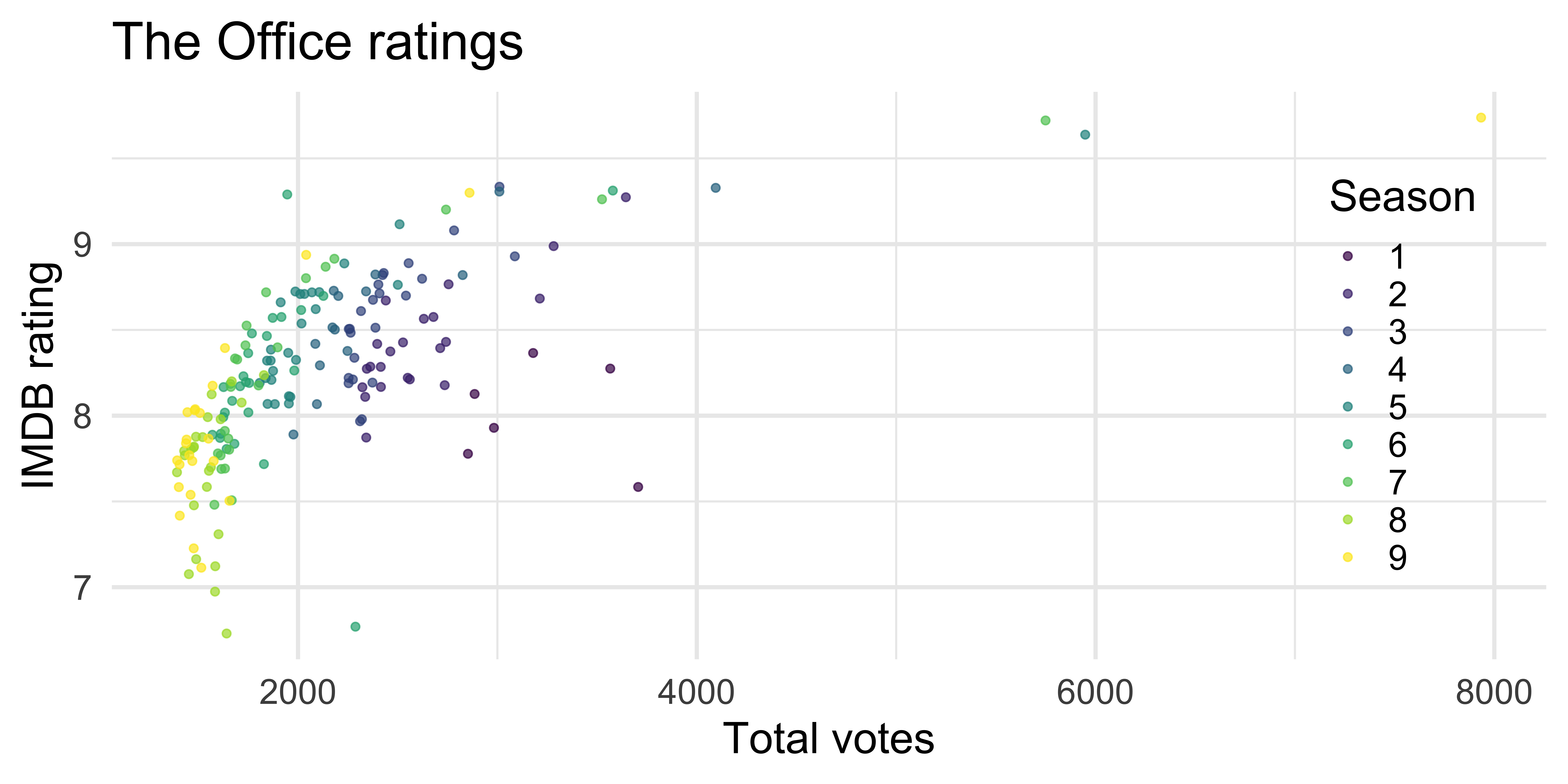
IMDB ratings vs. number of votes

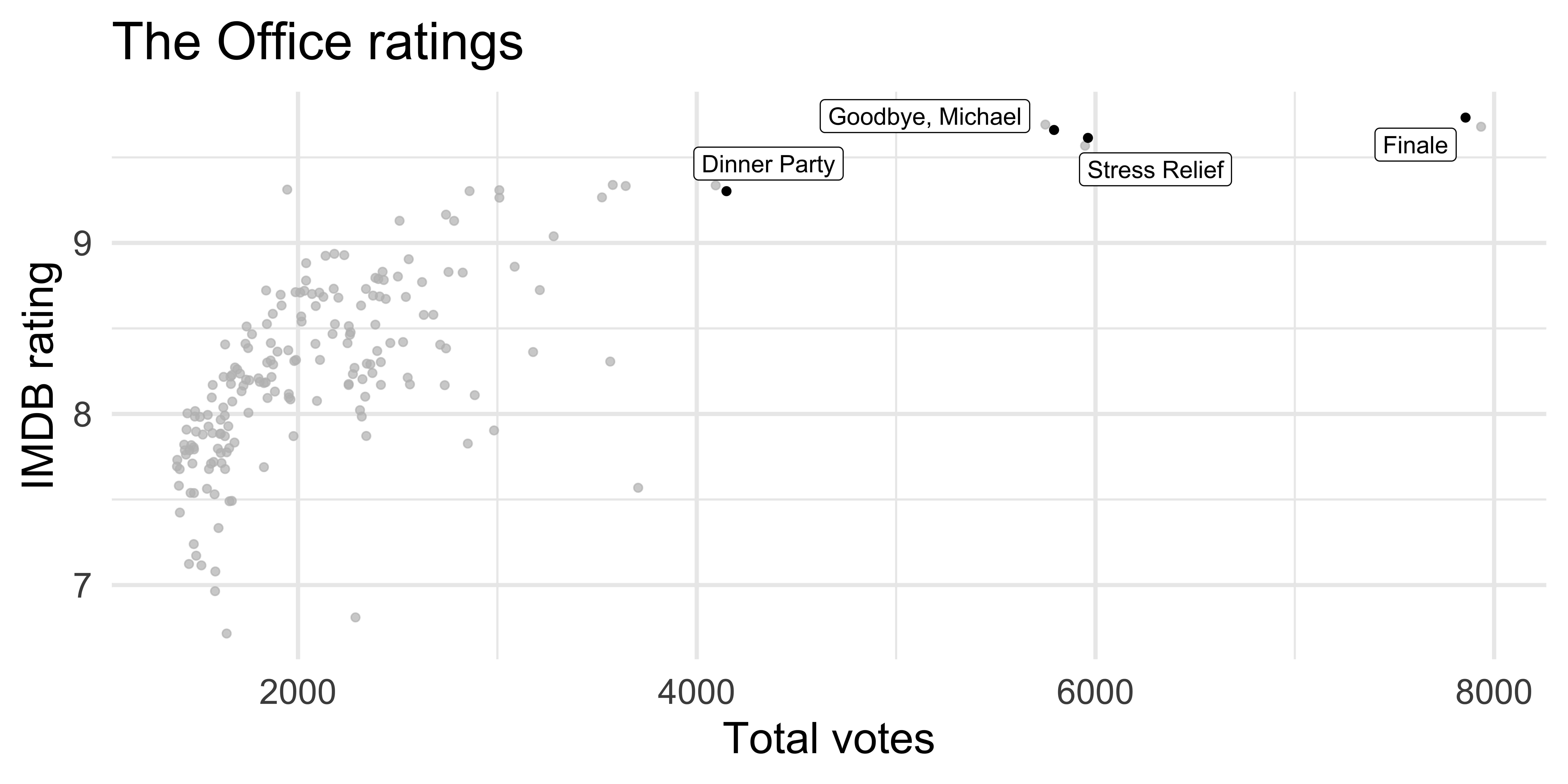
Outliers

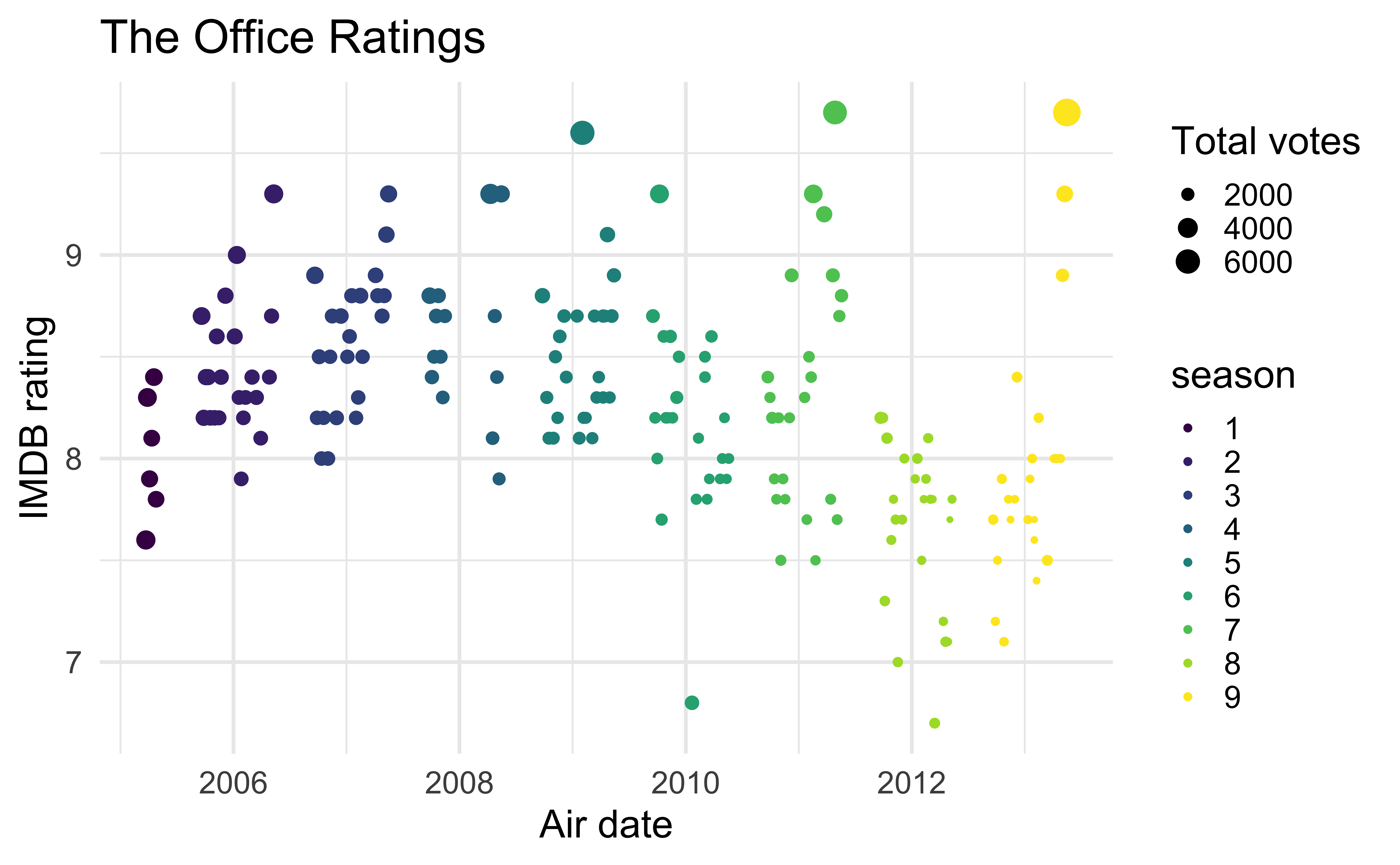
IMDB ratings vs. air date

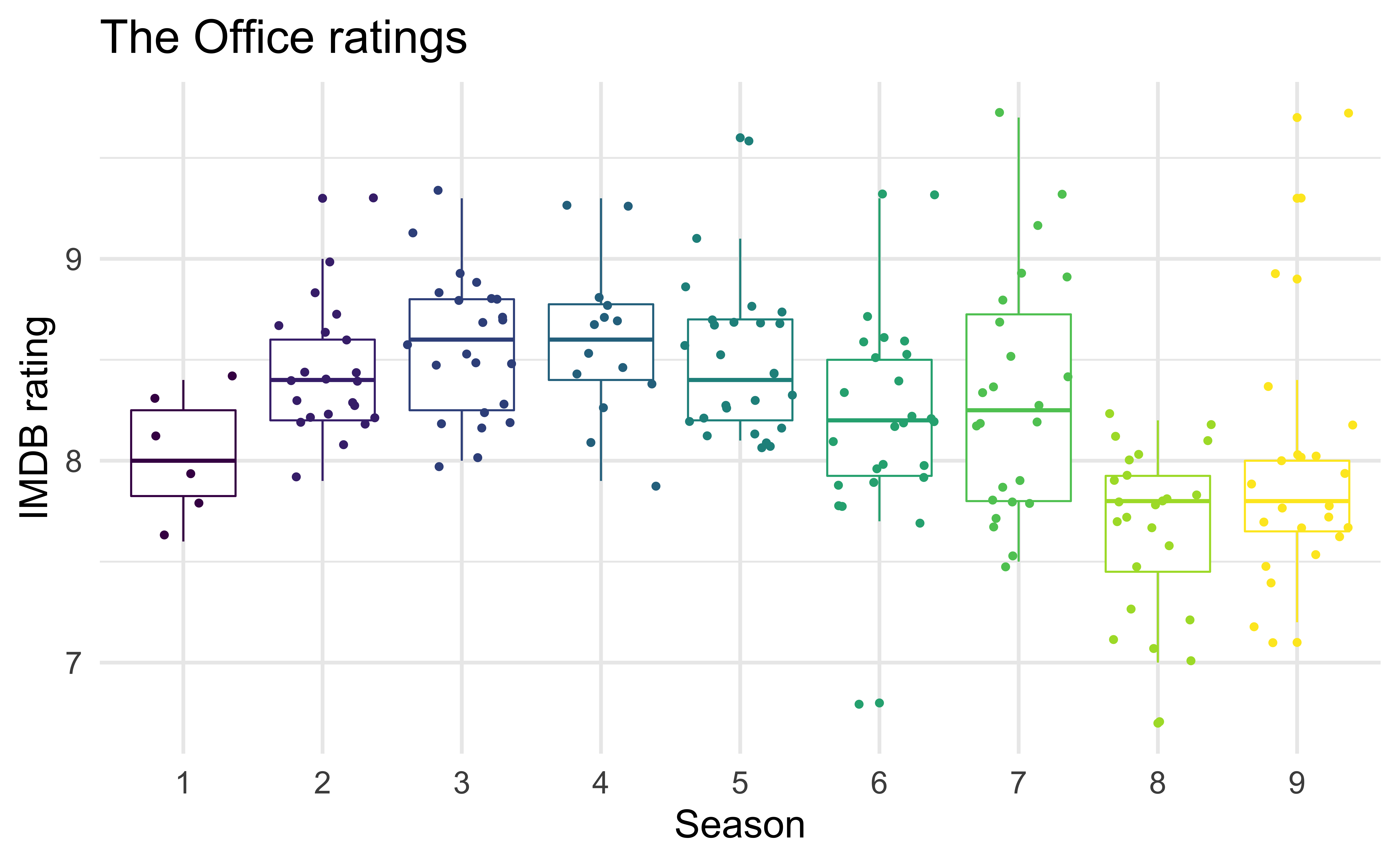
IMDB ratings vs. seasons

Modeling

Spending our data

• There are several steps to create a useful model: parameter estimation, model selection, performance assessment, etc.

• Doing all of this on the entire data we have available leaves us with no other data to assess our choices

• We can allocate specific subsets of data for different tasks, as opposed to allocating the largest possible amount to the model parameter estimation only (which is what we’ve done so far)

Train / test

Step 1: Create an initial split:

set.seed(123)
office_split <- initial_split(office_ratings) # prop = 3/4 by default

Step 2: Save training data

office_train <- training(office_split)
dim(office_train)

[1] 141   6

Step 3: Save testing data

office_test  <- testing(office_split)
dim(office_test)

[1] 47  6

Training data

office_train

# A tibble: 141 × 6
   season episode title               imdb_rating total_votes air_date  
    <dbl>   <dbl> <chr>                     <dbl>       <dbl> <date>    
 1      8      18 Last Day in Florida         7.8        1429 2012-03-08
 2      9      14 Vandalism                   7.6        1402 2013-01-31
 3      2       8 Performance Review          8.2        2416 2005-11-15
 4      9       5 Here Comes Treble           7.1        1515 2012-10-25
 5      3      22 Beach Games                 9.1        2783 2007-05-10
 6      7       1 Nepotism                    8.4        1897 2010-09-23
 7      3      15 Phyllis' Wedding            8.3        2283 2007-02-08
 8      9      21 Livin' the Dream            8.9        2041 2013-05-02
 9      9      18 Promos                      8          1445 2013-04-04
10      8      12 Pool Party                  8          1612 2012-01-19
# … with 131 more rows

Feature engineering

• We prefer simple (parsimonious) models when possible, but parsimony does not mean sacrificing accuracy (or predictive performance) in the interest of simplicity

• Variables that go into the model and how they are represented are just as critical to success of the model

• Feature engineering allows us to get creative with our predictors in an effort to make them more useful for our model (to increase its predictive performance)

Feature engineering with dplyr

office_train |>
  mutate(
    season = as_factor(season),
    month = lubridate::month(air_date),
    wday = lubridate::wday(air_date)
  )

# A tibble: 141 × 8
  season episode title               imdb_rating total_…¹ air_date   month  wday
  <fct>    <dbl> <chr>                     <dbl>    <dbl> <date>     <dbl> <dbl>
1 8           18 Last Day in Florida         7.8     1429 2012-03-08     3     5
2 9           14 Vandalism                   7.6     1402 2013-01-31     1     5
3 2            8 Performance Review          8.2     2416 2005-11-15    11     3
4 9            5 Here Comes Treble           7.1     1515 2012-10-25    10     5
5 3           22 Beach Games                 9.1     2783 2007-05-10     5     5
6 7            1 Nepotism                    8.4     1897 2010-09-23     9     5
# … with 135 more rows, and abbreviated variable name ¹​total_votes

Can you identify any potential problems with this approach?

Modeling workflow

• Create a recipe for feature engineering steps to be applied to the training data

• Fit the model to the training data after these steps have been applied

• Using the model estimates from the training data, predict outcomes for the test data

• Evaluate the performance of the model on the test data

Building recipes

Initiate a recipe

office_rec <- recipe(
  imdb_rating ~ .,    # formula
  data = office_train # data for cataloging names and types of variables
  )

office_rec

Recipe

Inputs:

      role #variables
   outcome          1
 predictor          5

Step 1: Alter roles

title isn’t a predictor, but we might want to keep it around as an ID

office_rec <- office_rec |>
  update_role(title, new_role = "ID")

office_rec

Recipe

Inputs:

      role #variables
        ID          1
   outcome          1
 predictor          4

Step 2: Add features

New features for day of week and month

office_rec <- office_rec |>
  step_date(air_date, features = c("dow", "month"))

office_rec

Recipe

Inputs:

      role #variables
        ID          1
   outcome          1
 predictor          4

Operations:

Date features from air_date

Step 3: Add more features

Identify holidays in air_date, then remove air_date

office_rec <- office_rec |>
  step_holiday(
    air_date, 
    holidays = c("USThanksgivingDay", "USChristmasDay", "USNewYearsDay", "USIndependenceDay"), 
    keep_original_cols = FALSE
  )

office_rec

Recipe

Inputs:

      role #variables
        ID          1
   outcome          1
 predictor          4

Operations:

Date features from air_date
Holiday features from air_date

Step 4: Convert numbers to factors

Convert season to factor

office_rec <- office_rec |>
  step_num2factor(season, levels = as.character(1:9))

office_rec

Recipe

Inputs:

      role #variables
        ID          1
   outcome          1
 predictor          4

Operations:

Date features from air_date
Holiday features from air_date
Factor variables from season

Step 5: Make dummy variables

Convert all nominal (categorical) predictors to factors

office_rec <- office_rec |>
  step_dummy(all_nominal_predictors())

office_rec

Recipe

Inputs:

      role #variables
        ID          1
   outcome          1
 predictor          4

Operations:

Date features from air_date
Holiday features from air_date
Factor variables from season
Dummy variables from all_nominal_predictors()

Step 6: Remove zero variance predictors

Remove all predictors that contain only a single value

office_rec <- office_rec |>
  step_zv(all_predictors())

office_rec

Recipe

Inputs:

      role #variables
        ID          1
   outcome          1
 predictor          4

Operations:

Date features from air_date
Holiday features from air_date
Factor variables from season
Dummy variables from all_nominal_predictors()
Zero variance filter on all_predictors()

Putting it all together

office_rec <- recipe(imdb_rating ~ ., data = office_train) |>
  # make title's role ID
  update_role(title, new_role = "ID") |>
  # extract day of week and month of air_date
  step_date(air_date, features = c("dow", "month")) |>
  # identify holidays and add indicators
  step_holiday(
    air_date, 
    holidays = c("USThanksgivingDay", "USChristmasDay", "USNewYearsDay", "USIndependenceDay"), 
    keep_original_cols = FALSE
  ) |>
  # turn season into factor
  step_num2factor(season, levels = as.character(1:9)) |>
  # make dummy variables
  step_dummy(all_nominal_predictors()) |>
  # remove zero variance predictors
  step_zv(all_predictors())

Putting it all together

office_rec

Recipe

Inputs:

      role #variables
        ID          1
   outcome          1
 predictor          4

Operations:

Date features from air_date
Holiday features from air_date
Factor variables from season
Dummy variables from all_nominal_predictors()
Zero variance filter on all_predictors()

Next step…

We will complete the workflow to fit a model predicting IMDB ratings that includes the following predictors:

• episode
• total_votes
• indicator variables for season
• indicator variables for day of week aired (created using air_date)
• indicator variables for month aired (created using air_date)

What feature will not end up in the final model? Why is it not included?

Recap

• Review: Training and testing splits
• Feature engineering with recipes