Variable transformations
Prof. Maria Tackett
Oct 12, 2022
Announcements
- Click here to fill out mid-semester survey by Friday.
- Lab 04 due:
- Thu, Oct 13, 11:59pm (Thu labs)
- Fri, Oct 14, 11:59pm (Fri labs)
- HW 02 due Wed, Oct 19, 11:59pm (released later today)
- Office hours resume tomorrow (Thursday)
- Click here for Week 07 activities.
Topics
Log transformation on the response variable
Log transformation on the predictor variable
Computational set up
Respiratory Rate vs. Age
A high respiratory rate can potentially indicate a respiratory infection in children. In order to determine what indicates a “high” rate, we first want to understand the relationship between a child’s age and their respiratory rate.
The data contain the respiratory rate for 618 children ages 15 days to 3 years. It was obtained from the Sleuth3 R package and is originally form a 1994 publication “Reference Values for Respiratory Rate in the First 3 Years of Life”.
Variables:
Age: age in monthsRate: respiratory rate (breaths per minute)
Rate vs. Age
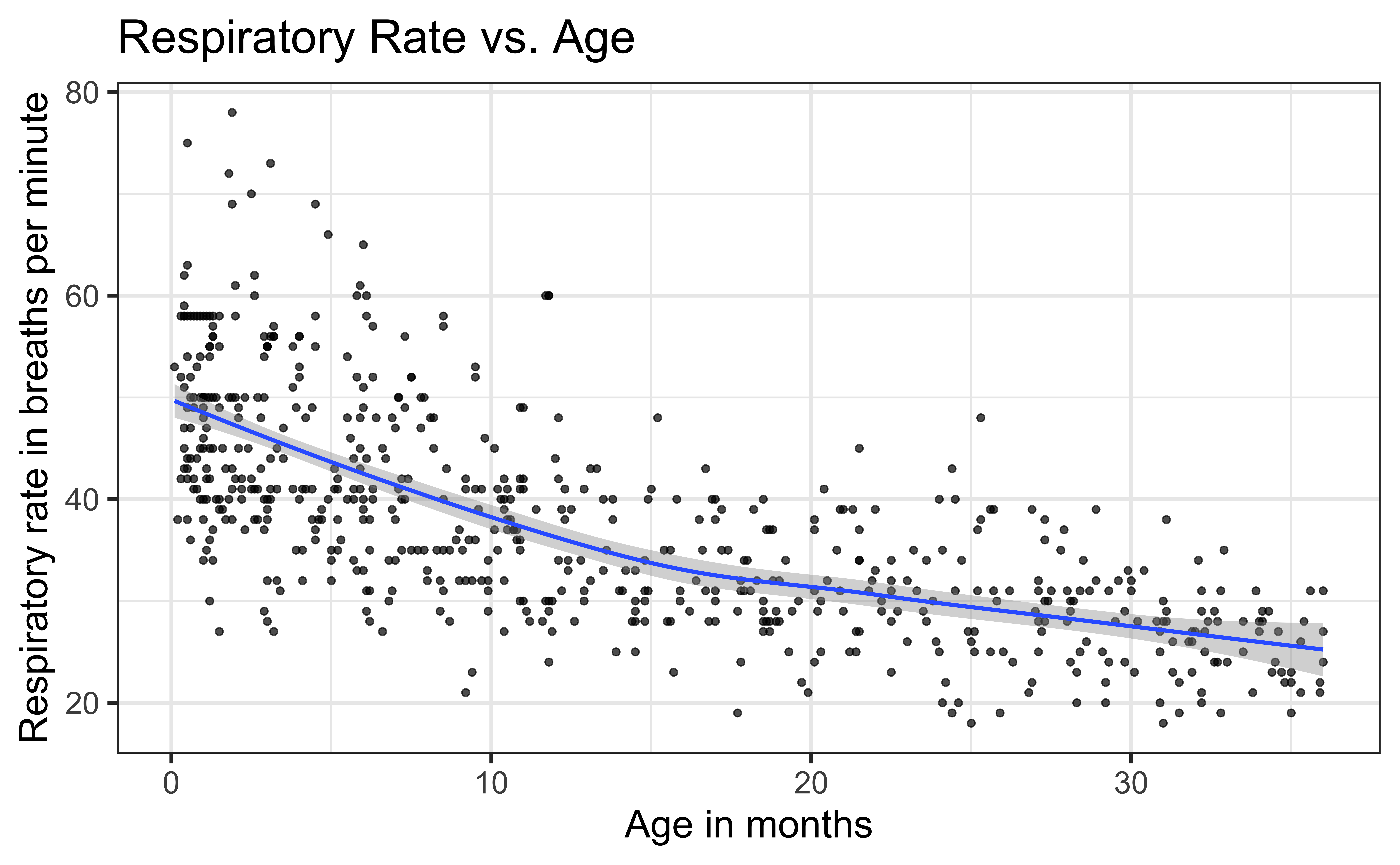
What do you notice in this plot?
Training + test sets
Model 1: Rate vs. Age
Model 1: Residuals
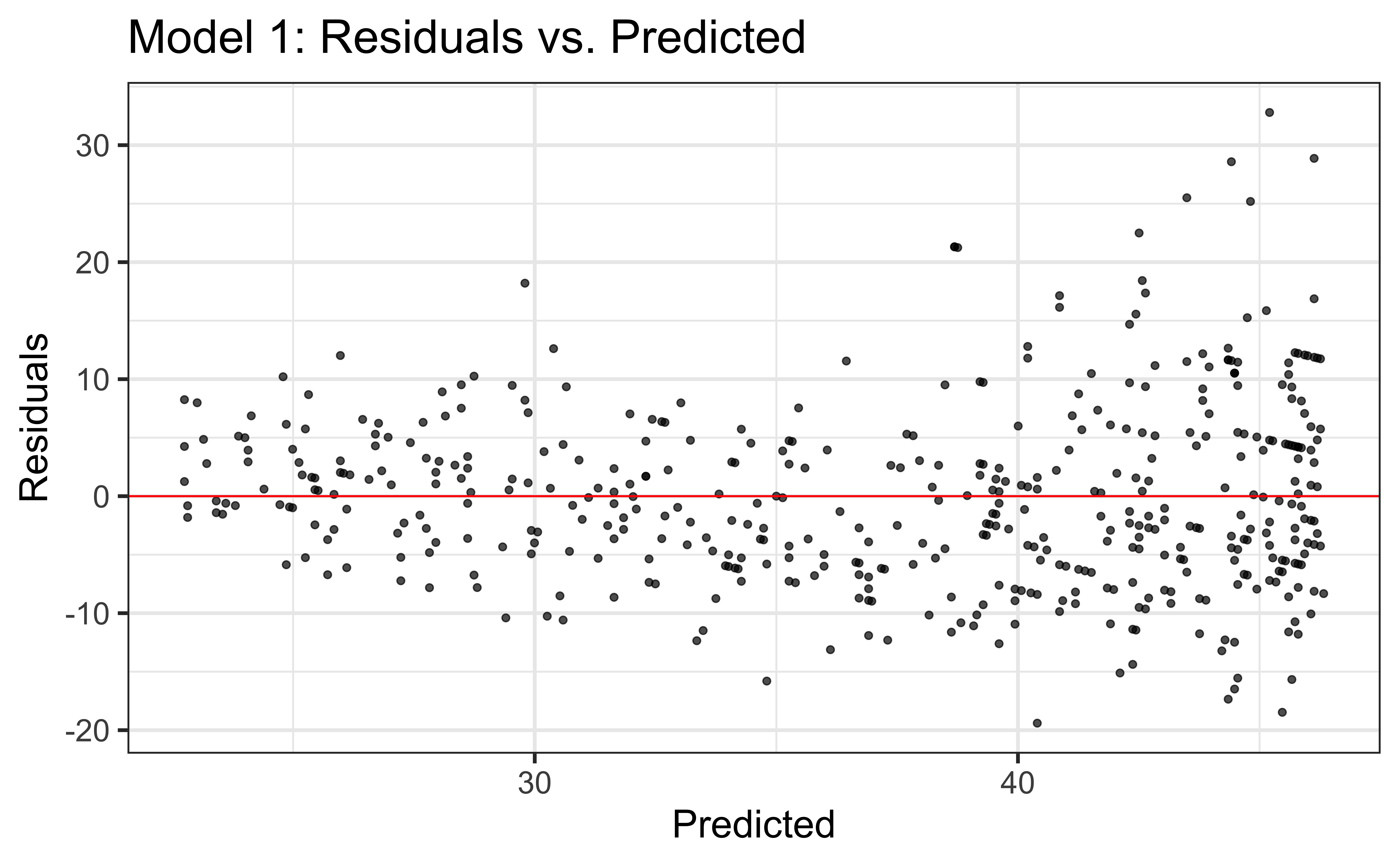
What do you notice in this plot?
Consider different transformations…
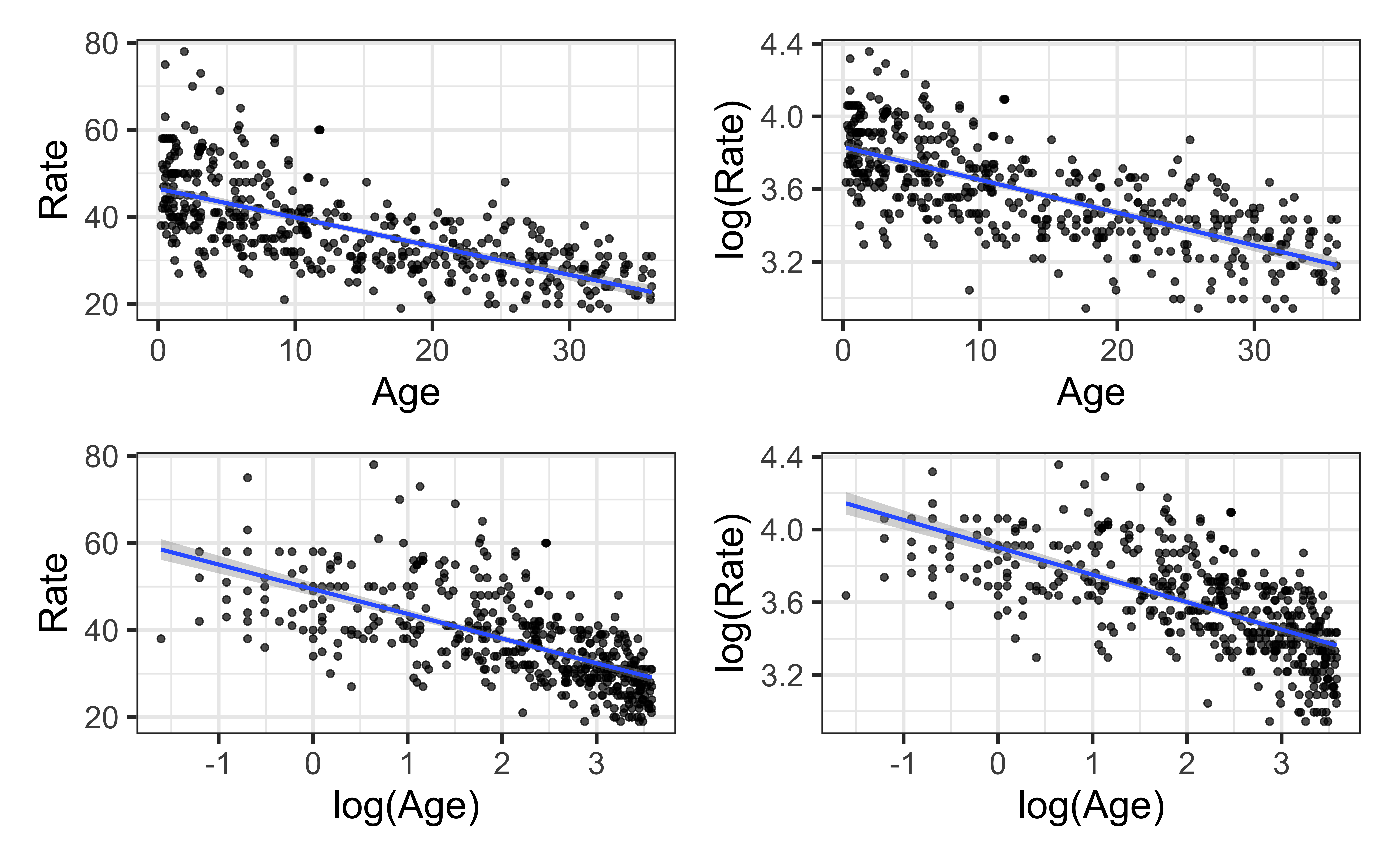
Log transformation on the response variable
Identifying a need to transform \(Y\)
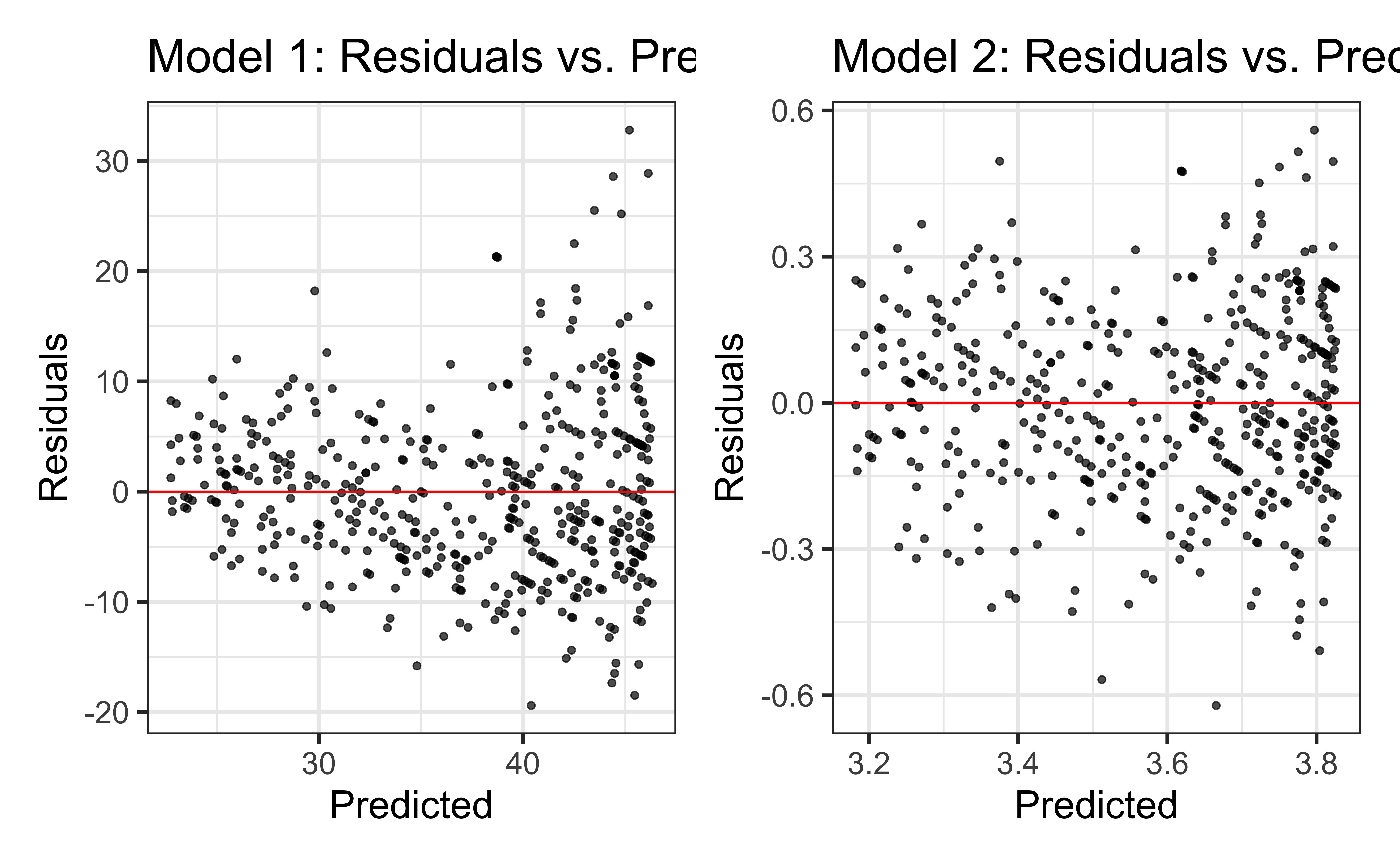
- Typically, a “fan-shaped” residual plot indicates the need for a transformation of the response variable \(Y\)
- There are multiple ways to transform a variable, e.g., \(\sqrt{Y}\), \(1/Y\), \(\log(Y)\).
- \(\log(Y)\) the most straightforward to interpret, so we use that transformation when possible
- When building a model:
- Choose a transformation and build the model on the transformed data
- Reassess the residual plots
- If the residuals plots did not sufficiently improve, try a new transformation!
Log transformation on \(Y\)
- If we apply a log transformation to the response variable, we want to estimate the parameters for the statistical model
\[ \log(Y) = \beta_0+ \beta_1 X + \epsilon, \hspace{10mm} \epsilon \sim N(0,\sigma^2_\epsilon) \]
- The regression equation is
\[\widehat{\log(Y)} = \hat{\beta}_0+ \hat{\beta}_1 X\]
Log transformation on \(Y\)
We want to interpret the model in terms of the original variable \(Y\), not \(\log(Y)\), so we need to write the model in terms of \(Y\)
\[\hat{Y} = \exp\{\hat{\beta}_0 + \hat{\beta}_1 X\} = \exp\{\hat{\beta}_0\}\exp\{\hat{\beta}_1X\}\]
\[\widehat{\text{Median}({Y|X})} = \exp\{\hat{\beta}_0\}\exp\{\hat{\beta}_1 X\}\]
Model interpretation
\[\hat{Y} = \exp\{\hat{\beta}_0 + \hat{\beta}_1 X\} = \exp\{\hat{\beta}_0\}\exp\{\hat{\beta}_1X\}\]
Intercept: When \(X=0\), the median of \(Y\) is expected to be \(\exp\{\hat{\beta}_0\}\)
Slope: For every one unit increase in \(X\), the median of \(Y\) is expected to multiply by a factor of \(\exp\{\hat{\beta}_1\}\)
Why is the interpretation in terms of a multiplicative change?
Why \(Median(Y|X)\) instead of \(\mu_{Y|X}\)
Suppose we have a set of values
Note: \(\overline{\log(x)} \neq \log(\bar{x})\)
Why \(Median(Y|X)\) instead of \(\mu_{Y|X}\)
Note: \(\text{Median}(\log(x)) = \log(\text{Median}(x))\)
Mean, Median, and log
\[\overline{\log(x)} \neq \log(\bar{x})\]
Mean and median of \(\log(Y)\)
Recall that \(Y = \beta_0 + \beta_1 X\) is the mean value of the response at the given value of the predictor \(X\). This doesn’t hold when we log-transform the response variable.
Mathematically, the mean of the logged values is not necessarily equal to the log of the mean value. Therefore at a given value of \(X\)
$$
\[\begin{aligned}\exp\{\text{Mean}(\log(Y|X))\} \neq \text{Mean}(Y|X) \\[5pt] \Rightarrow \exp\{\beta_0 + \beta_1 X\} \neq \text{Mean}(Y|X) \end{aligned}\]$$
Mean and median of \(\log(y)\)
- However, the median of the logged values is equal to the log of the median value. Therefore,
\[\exp\{\text{Median}(\log(Y|X))\} = \text{Median}(Y|X)\]
- If the distribution of \(\log(Y)\) is symmetric about the regression line, for a given value \(X\), we can expect \(Mean(Y)\) and \(Median(Y)\) to be approximately equal.
Model 2: log(Rate) vs. Age
| term | estimate | std.error | statistic | p.value |
|---|---|---|---|---|
| (Intercept) | 3.831 | 0.015 | 259.086 | 0 |
| Age | -0.018 | 0.001 | -21.243 | 0 |
Interpret the slope and intercept in the context of the data.
04:00
Model 2: Residuals
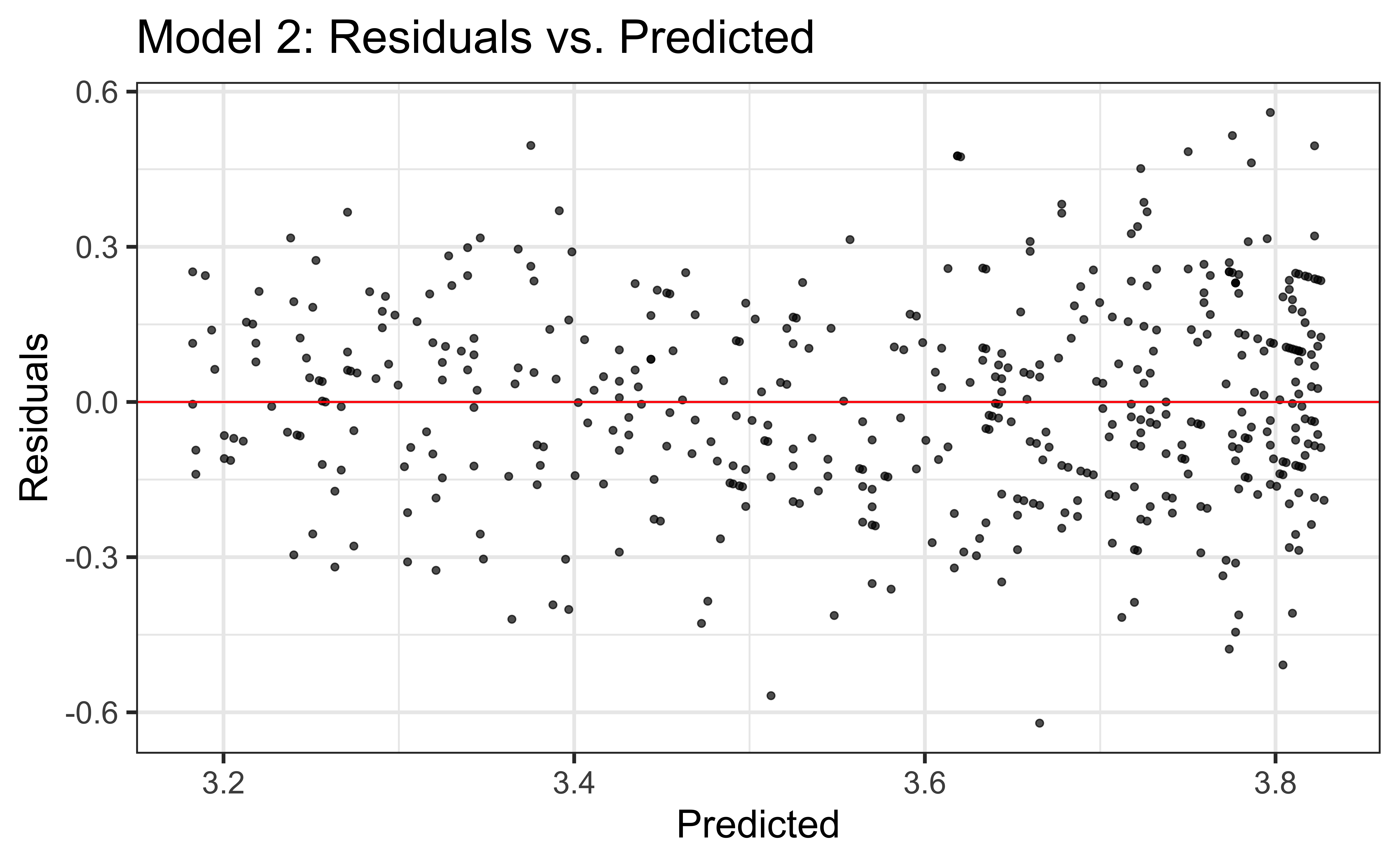
Compare residual plots
Log transformation on a predictor variable
Log Transformation on \(X\)
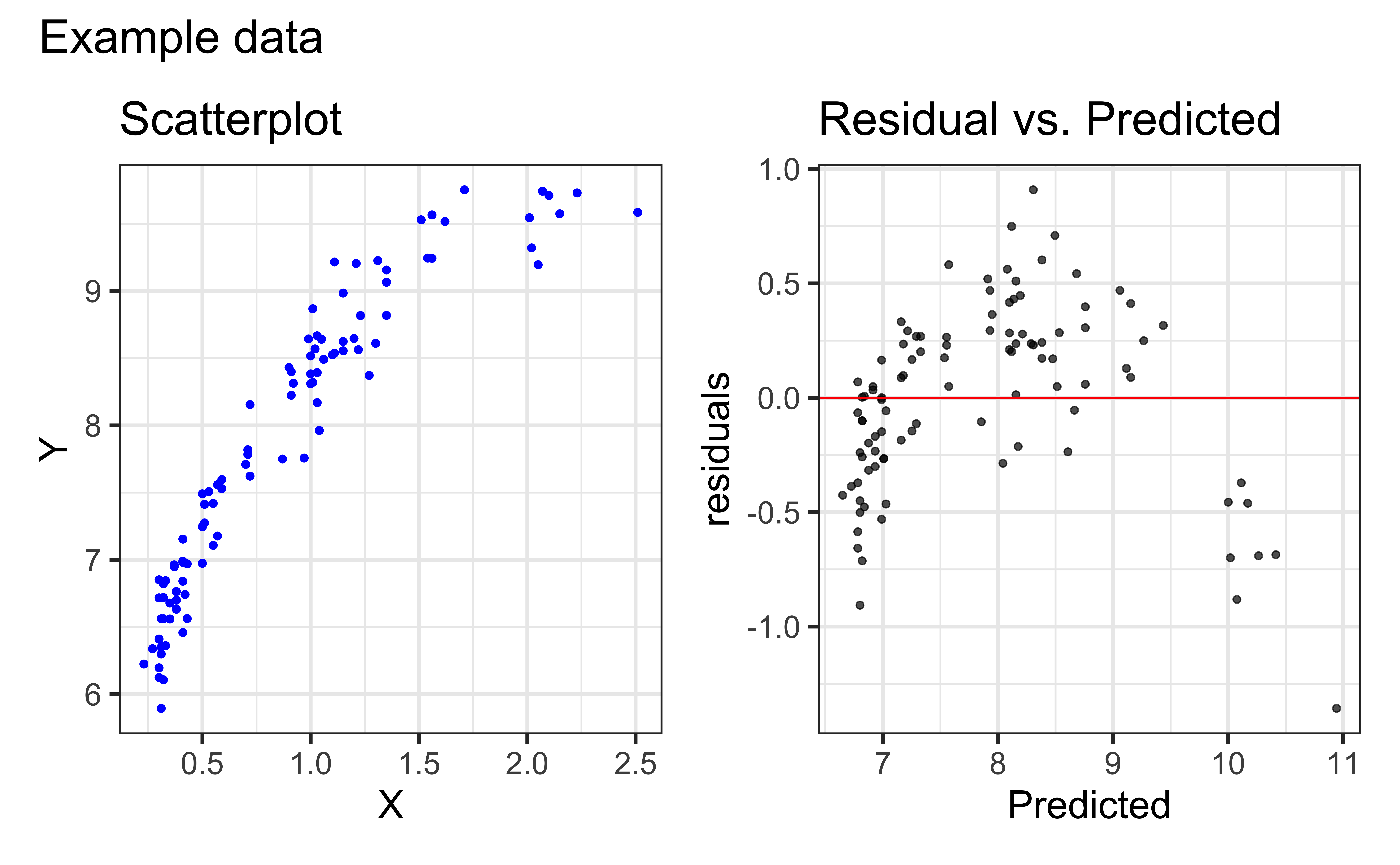
Try a transformation on \(X\) if the scatterplot shows some curvature but the variance is constant for all values of \(X\)
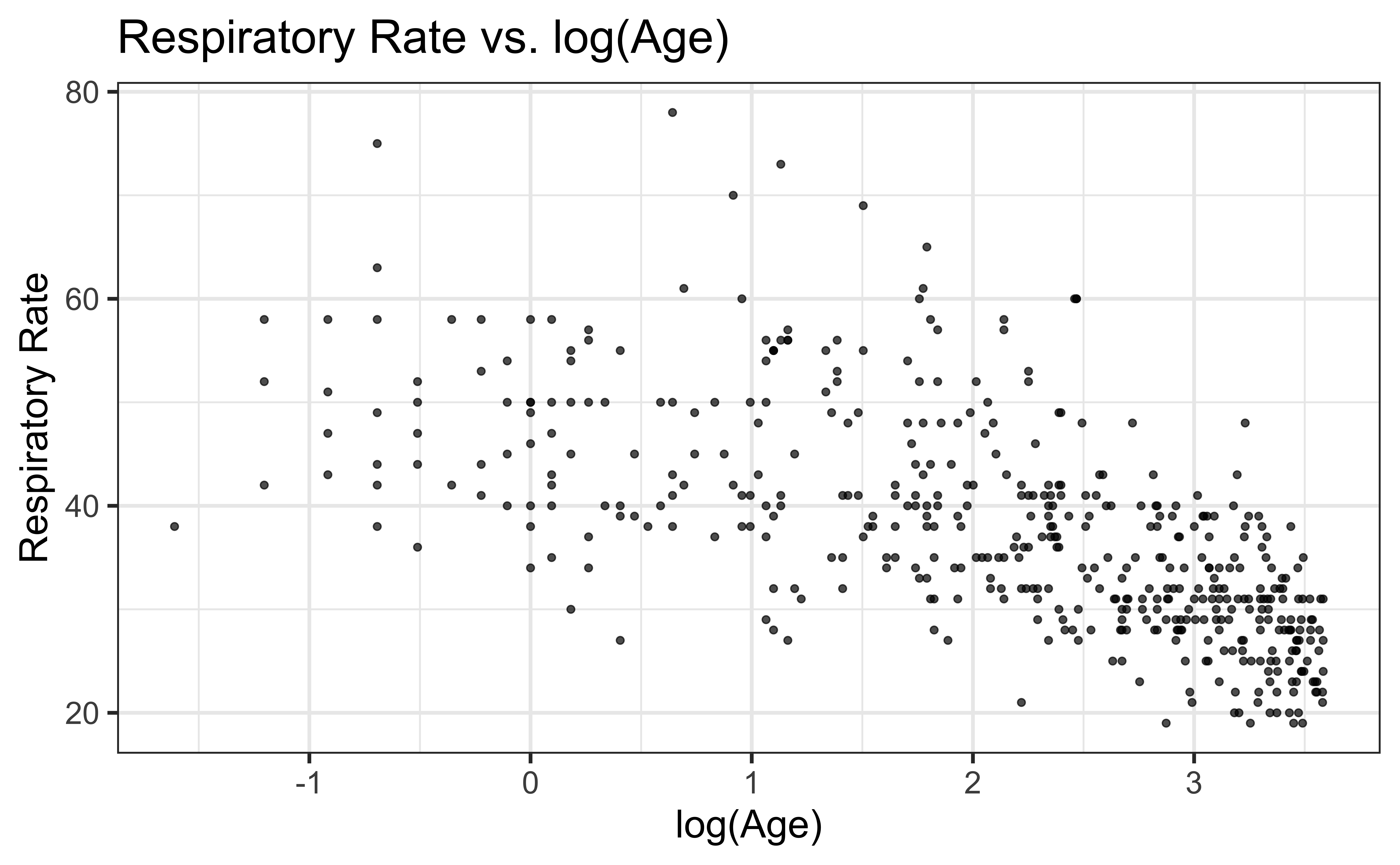
Rate vs. log(Age)
Model with Transformation on \(X\)
Suppose we have the following regression equation:
\[\hat{Y} = \hat{\beta}_0 + \hat{\beta}_1 \log(X)\]
Intercept: When \(X = 1\) \((\log(X) = 0)\), \(Y\) is expected to be \(\hat{\beta}_0\) (i.e. the mean of \(Y\) is \(\hat{\beta}_0\))
Slope: When \(X\) is multiplied by a factor of \(\mathbf{C}\), the mean of \(Y\) is expected to increase by \(\boldsymbol{\hat{\beta}_1}\mathbf{\log(C)}\) units
- Example: when \(X\) is multiplied by a factor of 2, \(Y\) is expected to increase by \(\boldsymbol{\hat{\beta}_1}\mathbf{\log(2)}\) units
Model 3: Rate vs. log(Age)
| term | estimate | std.error | statistic | p.value |
|---|---|---|---|---|
| (Intercept) | 49.397 | 0.755 | 65.436 | 0 |
| log_age | -5.668 | 0.311 | -18.248 | 0 |
Interpret the slope and intercept in the context of the data.
04:00
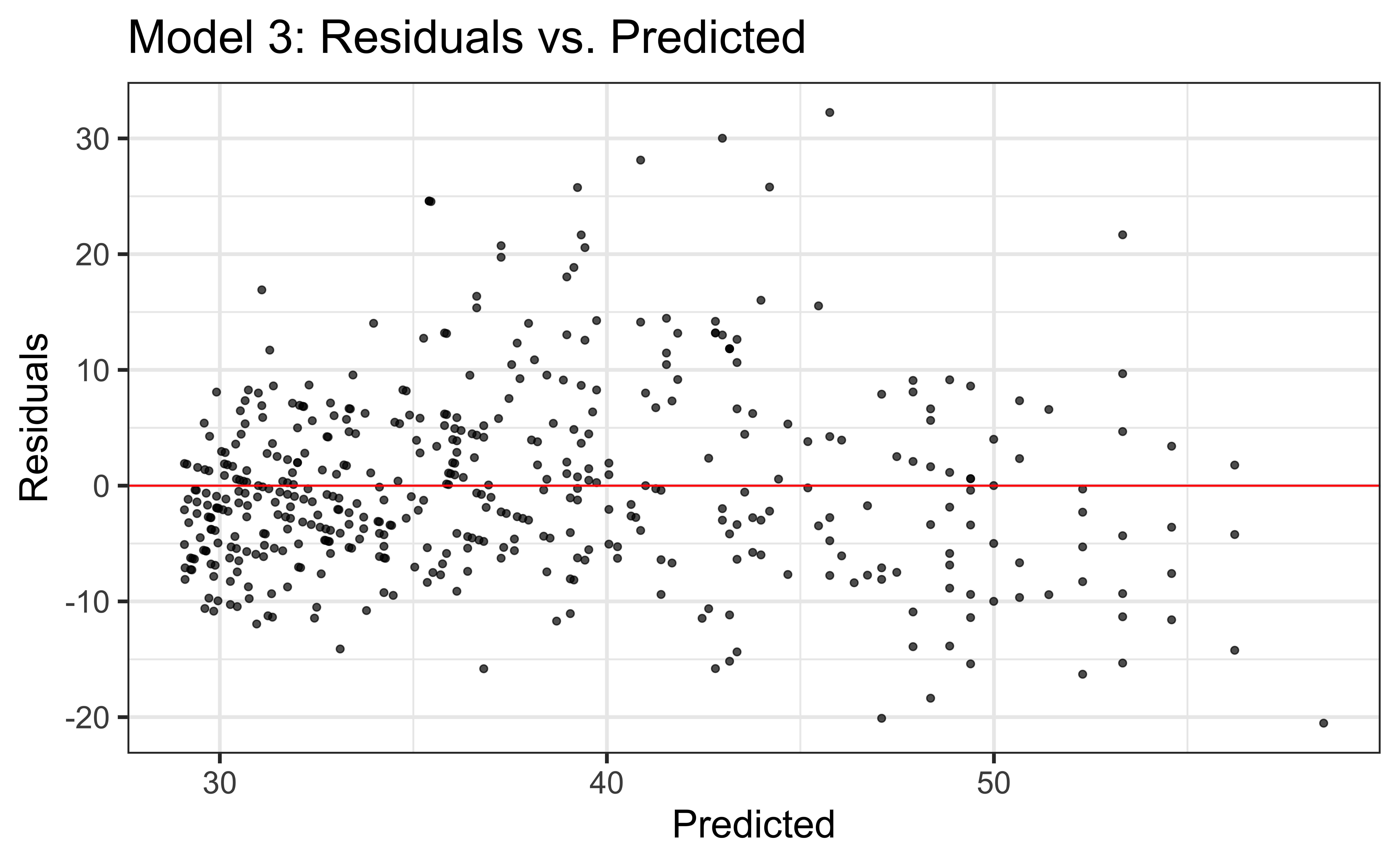
Model 3: Residuals
Choose a model
Recall the goal of the analysis:
In order to determine what indicates a “high” rate, we first want to understand the relationship between a child’s age and their respiratory rate.
Which is the preferred metric to compare the models - \(R^2\) or RMSE?
Compare models on testing data
| Rate vs. Age | log(Rate) vs. Age | Rate vs. log(Age) |
|---|---|---|
| 0.549 | 0.596 | 0.559 |
Which model would you choose?
Learn more
See Log Transformations in Linear Regression for more details about interpreting regression models with log-transformed variables.
