Variable transformations
Log-transformed predictor
Prof. Maria Tackett
Oct 17, 2022
Announcements
- HW 02 due Wed, Oct 19, 11:59pm
- Data Science Career Panel - October 19, 12 - 1pm, online
- Click here for Week 08 activities.
Mid-semester survey
Thank you to everyone who filled out a mid-semester survey!
Most helpful with learning
- Lectures / application exercises
- Office hours
Something to do more of to help with learning
- Reviewing assignments / common mistakes
- More examples /application exercises
Something the students can do more of / keep doing
- Review lecture notes
- Do assigned readings
- Attend office hours
Mid-semester survey
Other notes:
We will review office hours schedule to make sure they are scheduled during times that don’t have major conflicts
Grading
Wording in statistics matters! For example - these are two different statements:
- Correct: For every one month in age, we expect the respiratory rate to decrease by 0.659 breaths per minute, on average.
- Incorrect: For every one month in age, the respiratory rate will decrease by 0.659 breaths per minute.
Full credit is awarded for (1) using the most appropriate methods (e.g., appropriate summary statistics given a distribution), (2) comprehensively and accurately justifying response, (3) consistency in response and explanation.
There is an example in the lecture notes, application exercises, and/or readings.
Regrade requests
- Dates they are available in email from Gradescope
- Review solutions and ask during office hours first
- Do not submit regrade requests to dispute point values
- Question is completely regraded by Prof. Tackett or Head TA
- Policy in syllabus
Topics
Log transformation on the response variable
Log transformation on the predictor variable
Computational set up
Recap
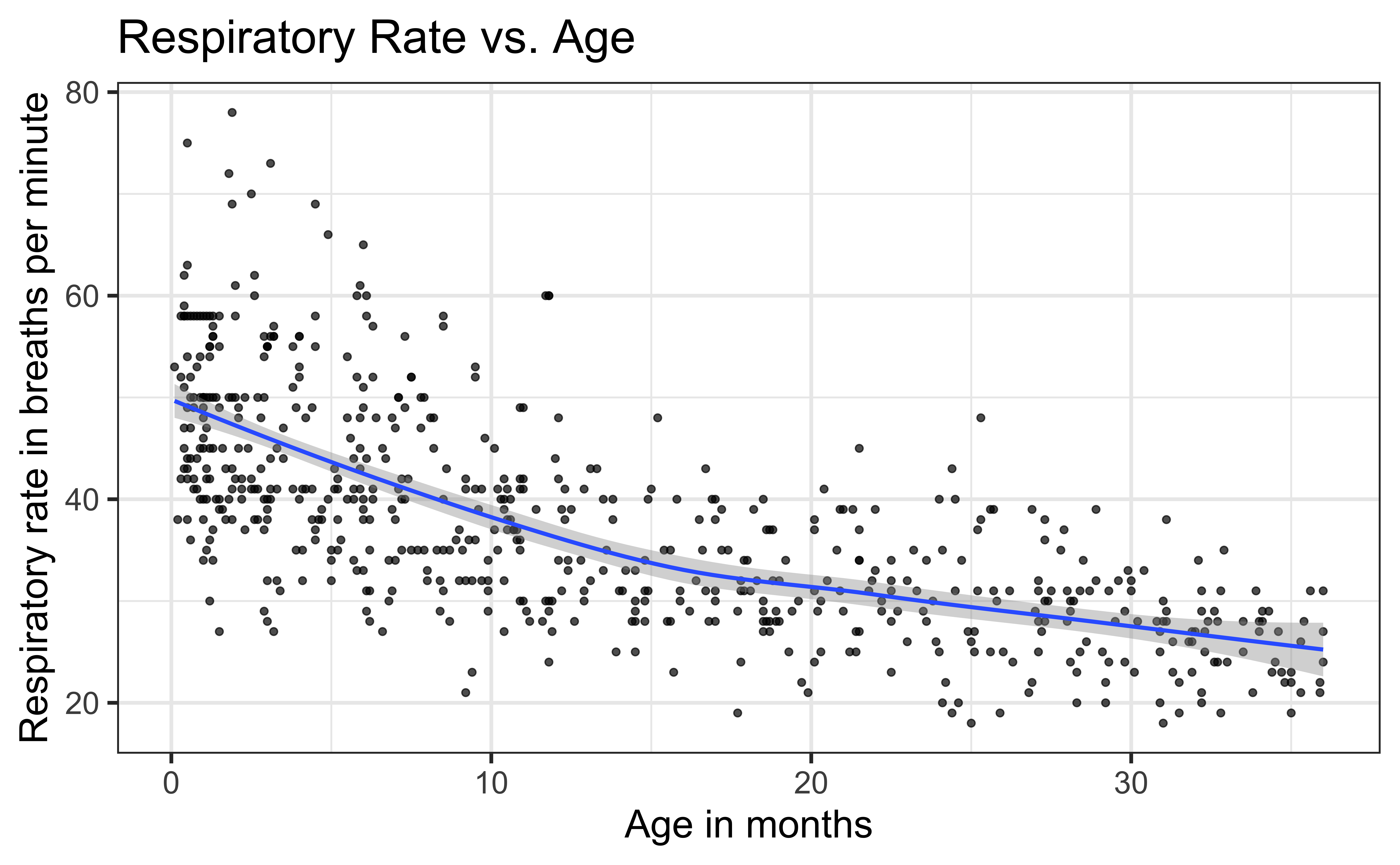
Respiratory Rate vs. Age
A high respiratory rate can potentially indicate a respiratory infection in children. In order to determine what indicates a “high” rate, we first want to understand the relationship between a child’s age and their respiratory rate.
The data contain the respiratory rate for 618 children ages 15 days to 3 years. It was obtained from the Sleuth3 R package and is originally form a 1994 publication “Reference Values for Respiratory Rate in the First 3 Years of Life”.
Variables:
Age: age in monthsRate: respiratory rate (breaths per minute)
Rate vs. Age
Training + test sets
Model 1: Rate vs. Age
Model 1: Residuals
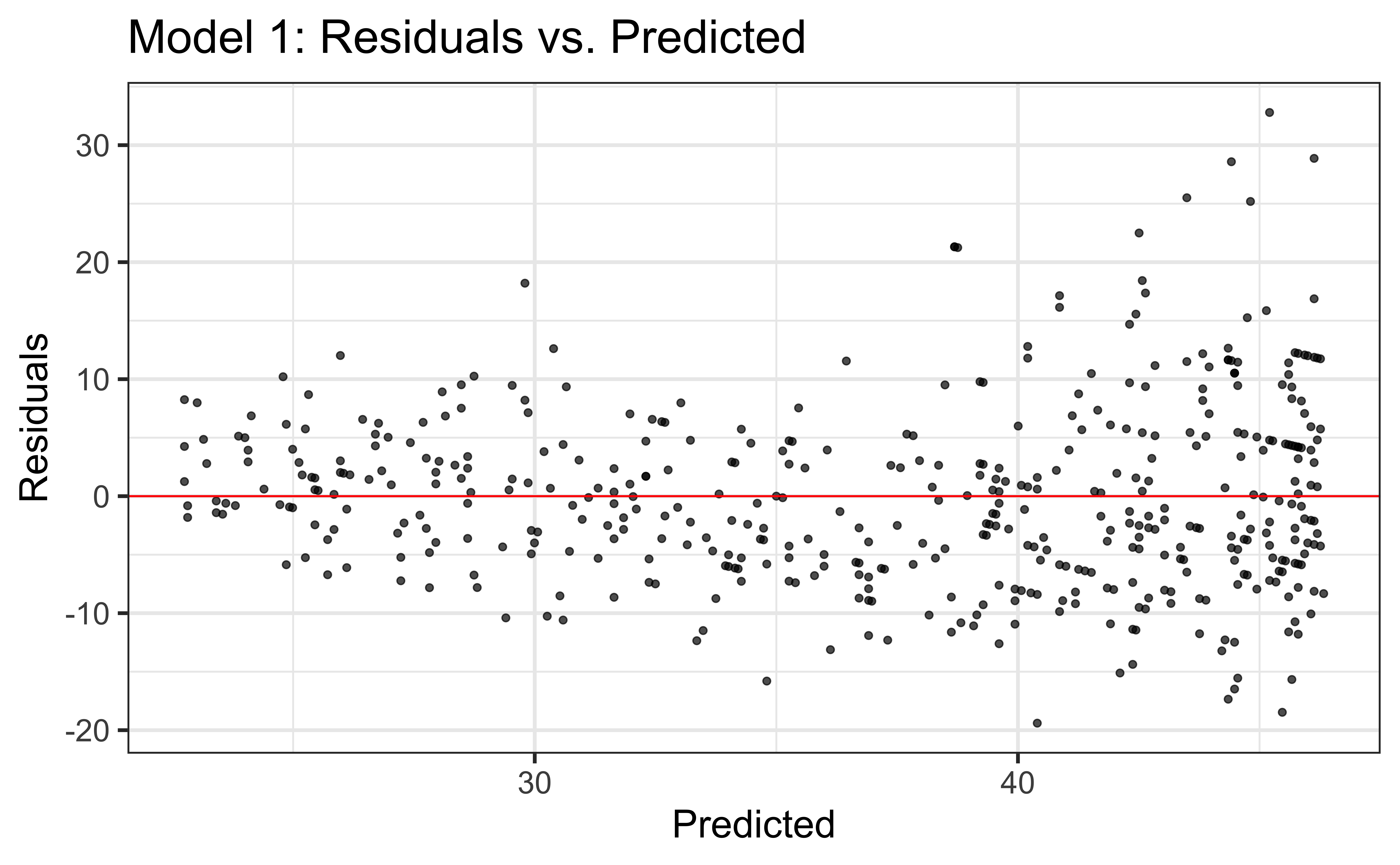
Consider different transformations…
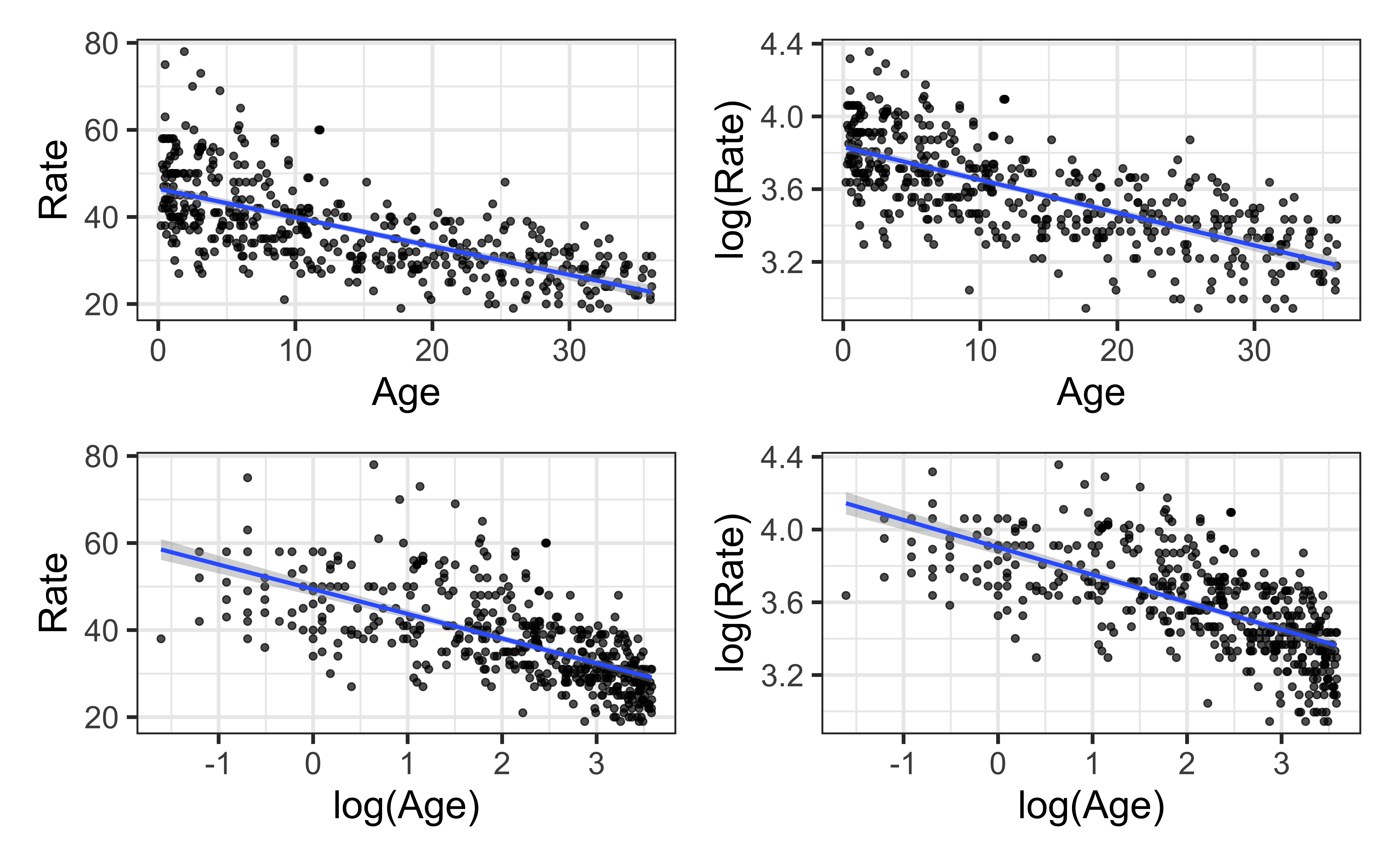
Model 2: log(Rate) vs. Age
| term | estimate | std.error | statistic | p.value |
|---|---|---|---|---|
| (Intercept) | 3.831 | 0.015 | 259.086 | 0 |
| Age | -0.018 | 0.001 | -21.243 | 0 |
Slope: For each additional month in a child’s age, the median respiratory rate is expected to multiply by a factor of 0.982 [exp(-0.018)].
Intercept: The median respiratory rate for children who are 0 months old is expected to be 29.4 [exp(3.381)].
Model 2: Residuals
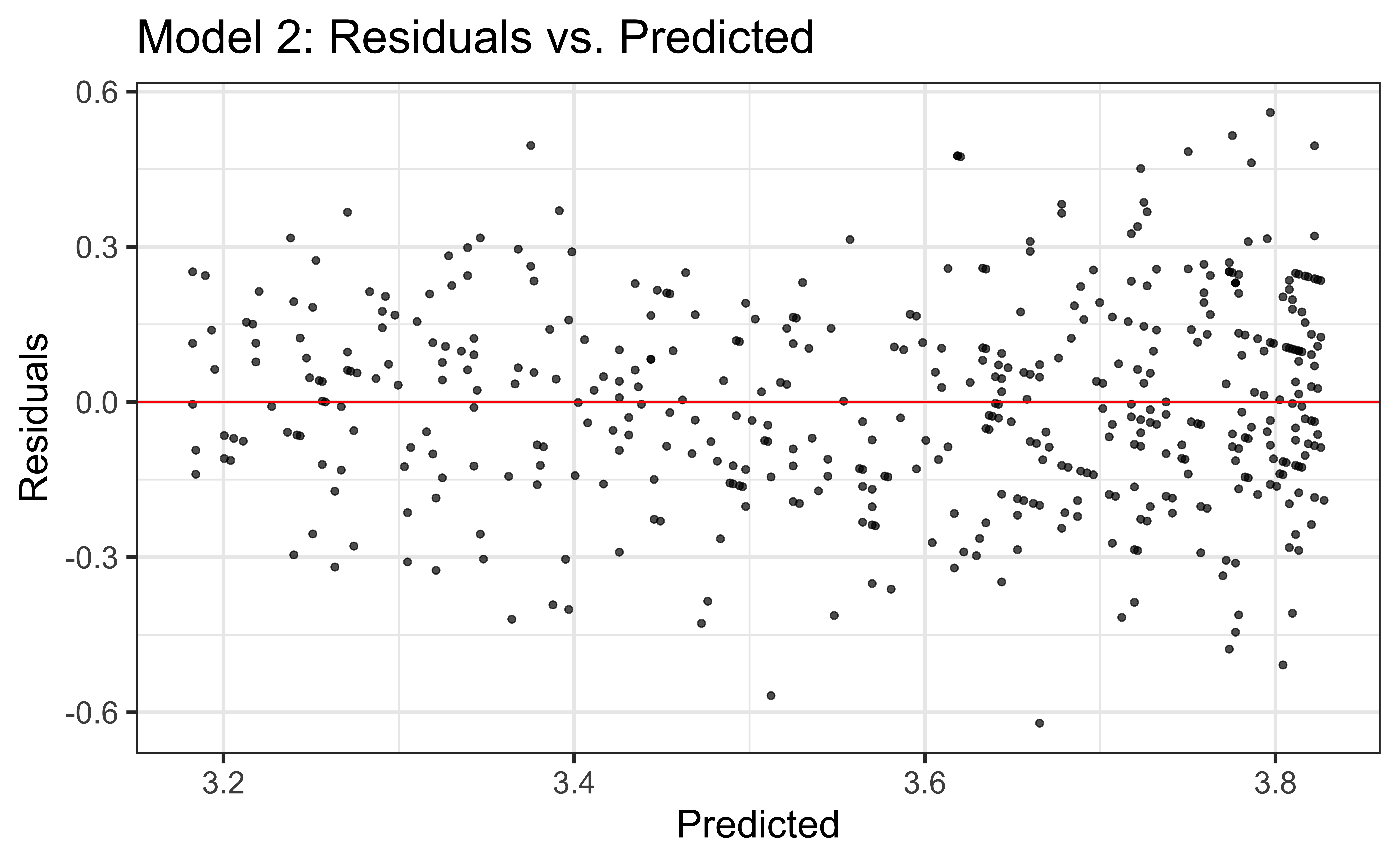
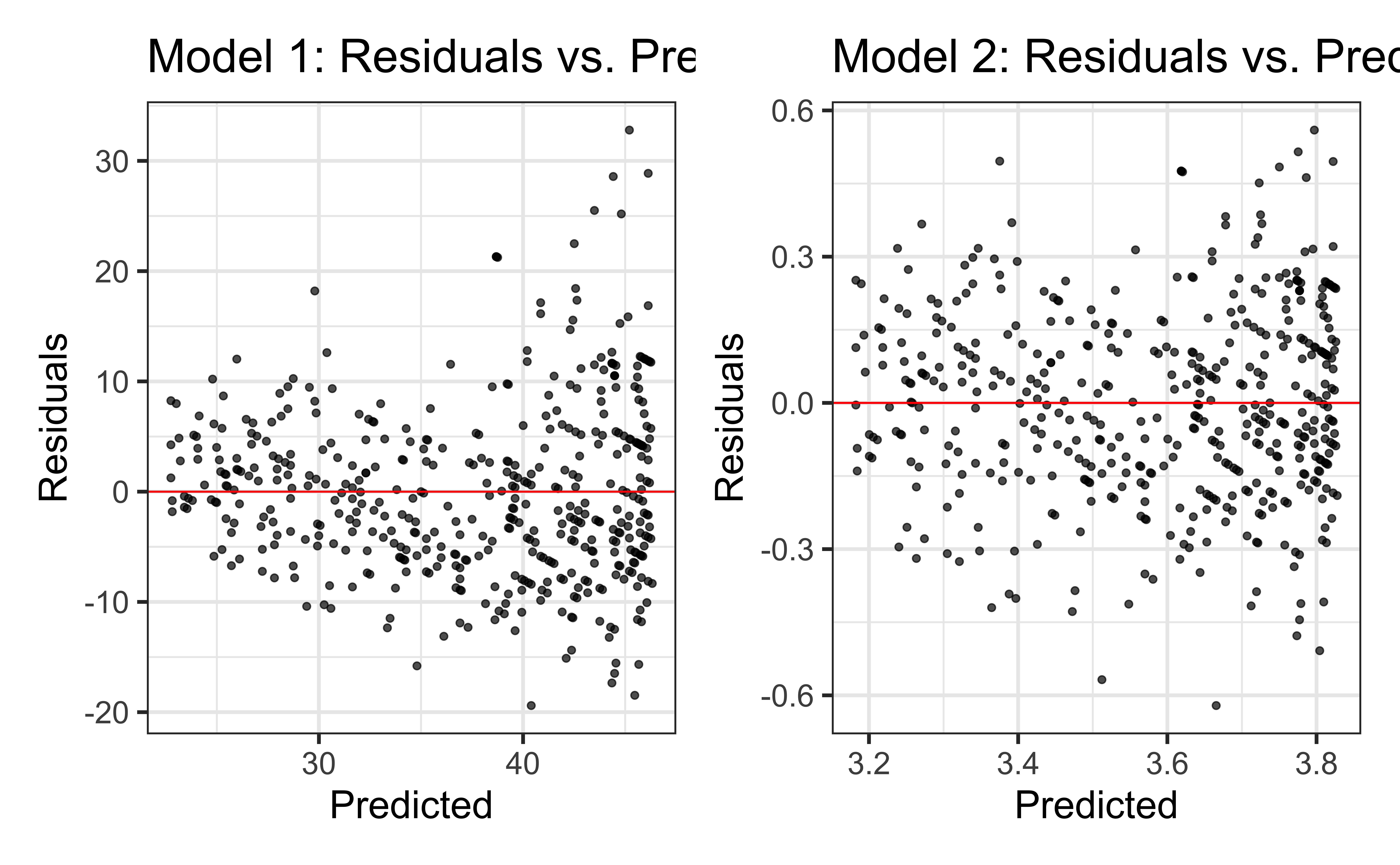
Compare residual plots
Log transformation on a predictor variable
Log Transformation on \(X\)
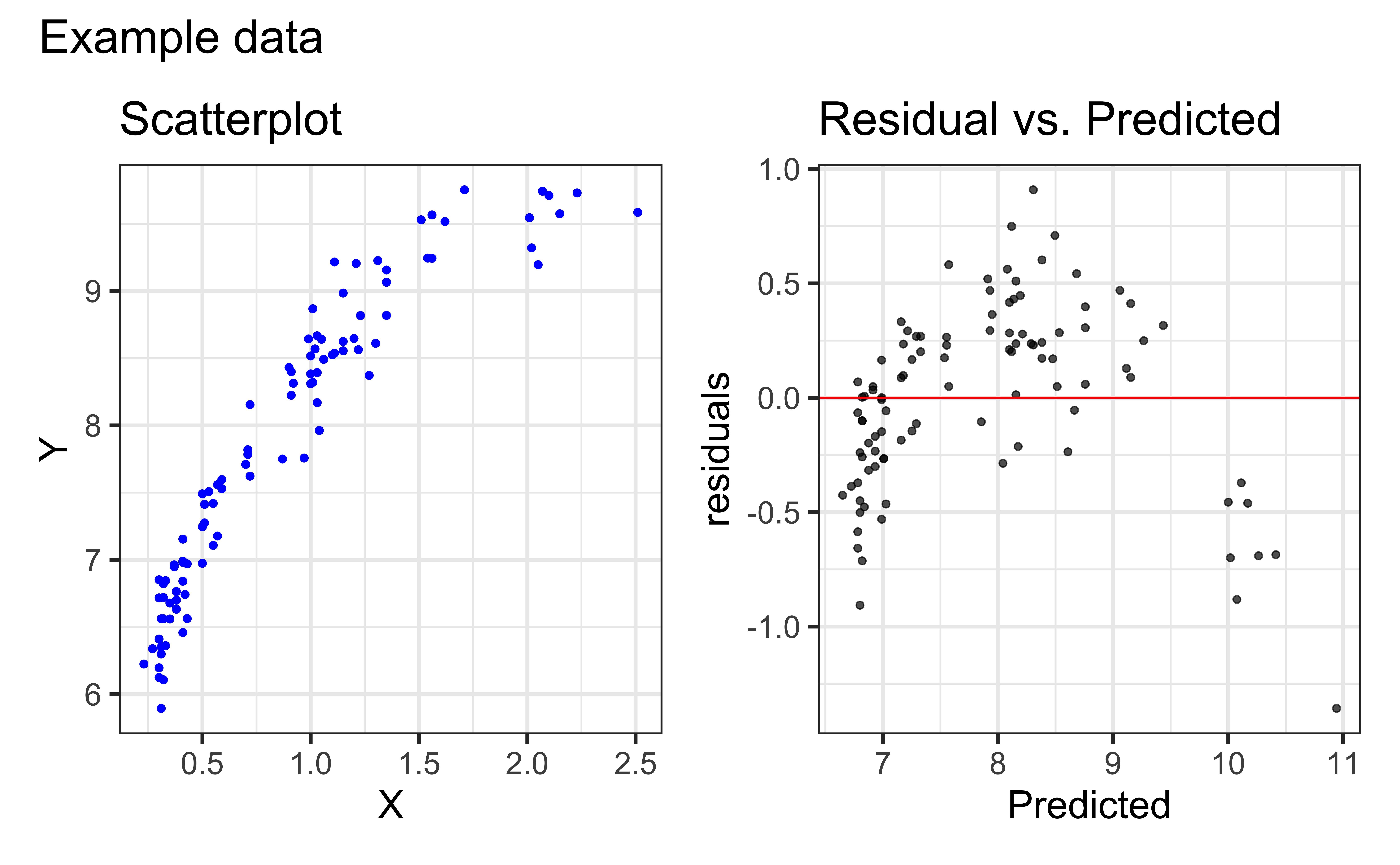
Try a transformation on \(X\) if the scatterplot shows some curvature but the variance is constant for all values of \(X\)
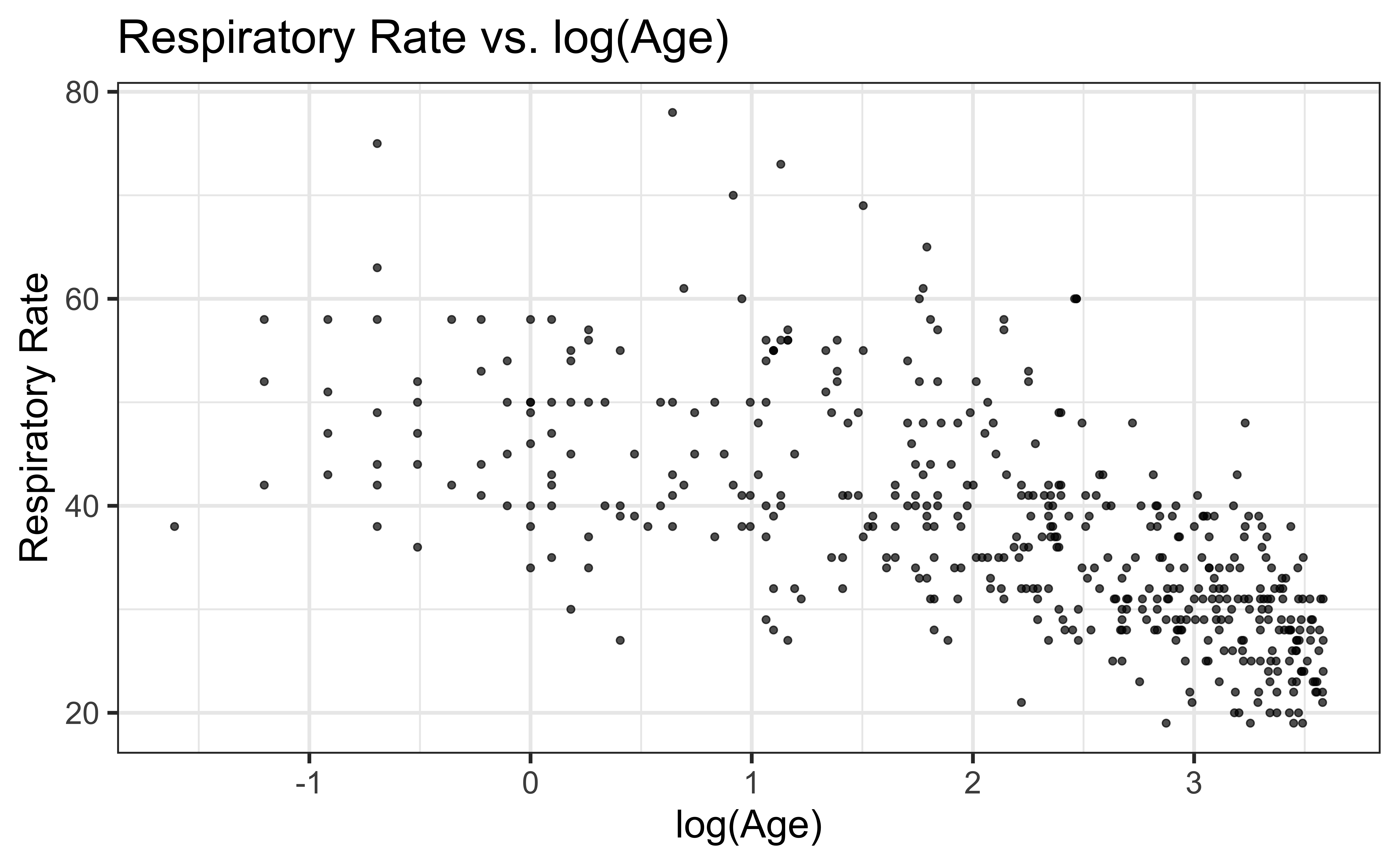
Rate vs. log(Age)
Model with Transformation on \(X\)
Suppose we have the following regression equation:
\[\hat{Y} = \hat{\beta}_0 + \hat{\beta}_1 \log(X)\]
Intercept: When \(X = 1\) \((\log(X) = 0)\), \(Y\) is expected to be \(\hat{\beta}_0\) (i.e. the mean of \(Y\) is \(\hat{\beta}_0\))
Slope: When \(X\) is multiplied by a factor of \(\mathbf{C}\), the mean of \(Y\) is expected to increase by \(\boldsymbol{\hat{\beta}_1}\mathbf{\log(C)}\) units
- Example: when \(X\) is multiplied by a factor of 2, \(Y\) is expected to increase by \(\boldsymbol{\hat{\beta}_1}\mathbf{\log(2)}\) units
Model 3: Rate vs. log(Age)
| term | estimate | std.error | statistic | p.value |
|---|---|---|---|---|
| (Intercept) | 49.397 | 0.755 | 65.436 | 0 |
| log_age | -5.668 | 0.311 | -18.248 | 0 |
Interpret the slope and intercept in the context of the data.
04:00
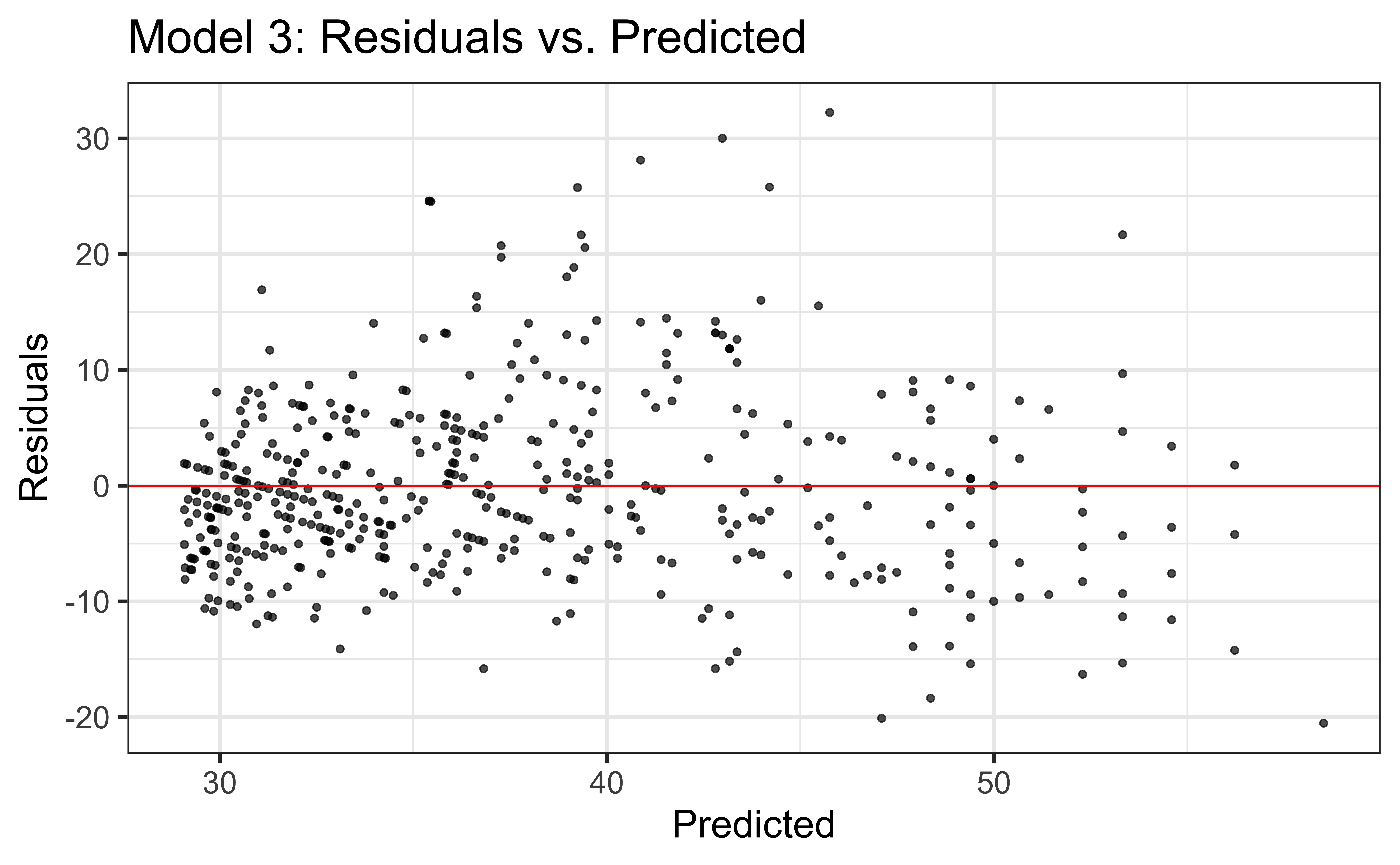
Model 3: Residuals
Choose a model
Recall the goal of the analysis:
In order to determine what indicates a “high” rate, we first want to understand the relationship between a child’s age and their respiratory rate.
Which is the preferred metric to compare the models - \(R^2\) or RMSE?
Compare models on testing data
| Rate vs. Age | log(Rate) vs. Age | Rate vs. log(Age) |
|---|---|---|
| 0.549 | 0.596 | 0.559 |
Which model would you choose?
Learn more
See Log Transformations in Linear Regression for more details about interpreting regression models with log-transformed variables.
