| term | estimate | std.error | statistic | p.value |
|---|---|---|---|---|
| (Intercept) | -14.676 | 1.881 | -7.804 | 0.000 |
| islandDream | -0.892 | 0.359 | -2.481 | 0.013 |
| islandTorgersen | 18.132 | 822.821 | 0.022 | 0.982 |
| bill_depth_mm | 0.836 | 0.113 | 7.416 | 0.000 |
Logistic Regression: Prediction + classification
Prof. Maria Tackett
Nov 09, 2022
Announcements
Aaditya’s office hours permanently moved to Wed 6 - 8pm
- New time reflected on website and Sakai
See Week 11 activities
Odds ratios practice
Let’s take a look at one of the models from Lab 06.
Interpret the coefficient of
bill_depth_mmin terms of the odds a penguin is from Adelie species.Interpret the coefficient of
islandDreamin terms of the odds a penguin is from Adelie species.
03:00
Topics
- Building predictive logistic regression models
- Sensitivity and specificity
- Making classification decisions
Computational setup
Data
openintro::email
These data represent incoming emails for the first three months of 2012 for an email account.
- Outcome:
spam- Indicator for whether the email was spam. - Predictors:
spam,to_multiple,from,cc,sent_email,time,image,attach,dollar,winner,inherit,viagra,password,num_char,line_breaks,format,re_subj,exclaim_subj,urgent_subj,exclaim_mess,number.
Click here for more detailed information on the variables.
Training and testing split
# Fix random numbers by setting the seed
# Enables analysis to be reproducible when random numbers are used
set.seed(1109)

# Put 75% of the data into the training set
email_split <- initial_split(email)

# Create data frames for the two sets
email_train <- training(email_split)
email_test  <- testing(email_split)
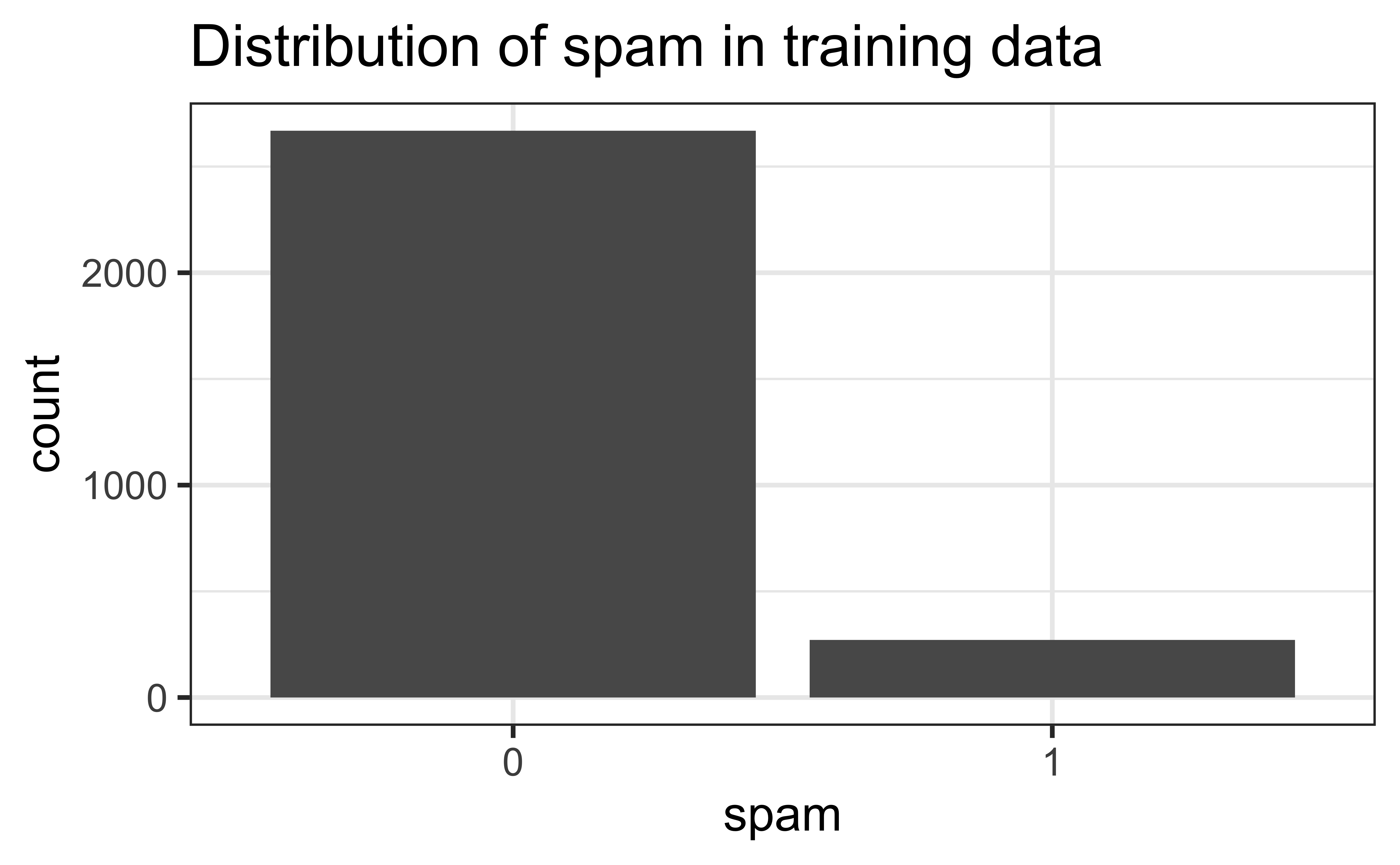
Exploratory data analysis
The sample is unbalanced with respect to spam.
Reminder: Modeling workflow
Create a recipe for feature engineering steps to be applied to the training data
Fit the model to the training data after these steps have been applied
- Use cross-validation if deciding between multiple models
Using the model estimates from the training data, predict outcomes for the test data
Evaluate the performance of the model on the test data
Start with a recipe
Initiate a recipe
# A tibble: 21 × 4
   variable     type    role      source
   <chr>        <chr>   <chr>     <chr>
 1 to_multiple  nominal predictor original
 2 from         nominal predictor original
 3 cc           numeric predictor original
 4 sent_email   nominal predictor original
 5 time         date    predictor original
 6 image        numeric predictor original
 7 attach       numeric predictor original
 8 dollar       numeric predictor original
 9 winner       nominal predictor original
10 inherit      numeric predictor original
11 viagra       numeric predictor original
12 password     numeric predictor original
13 num_char     numeric predictor original
14 line_breaks  numeric predictor original
15 format       nominal predictor original
16 re_subj      nominal predictor original
17 exclaim_subj numeric predictor original
18 urgent_subj  nominal predictor original
19 exclaim_mess numeric predictor original
20 number       nominal predictor original
21 spam         nominal outcome   original
Remove certain variables
Recipe

Inputs:

      role #variables
   outcome          1
 predictor         20

Operations:

Variables removed from, sent_email
Feature engineer date
Recipe

Inputs:

      role #variables
   outcome          1
 predictor         20

Operations:

Variables removed from, sent_email
Date features from time
Variables removed time
Discretize numeric variables
Recipe

Inputs:

      role #variables
   outcome          1
 predictor         20

Operations:

Variables removed from, sent_email
Date features from time
Variables removed time
Cut numeric for cc, attach, dollar
Create dummy variables
Recipe

Inputs:

      role #variables
   outcome          1
 predictor         20

Operations:

Variables removed from, sent_email
Date features from time
Variables removed time
Cut numeric for cc, attach, dollar
Dummy variables from all_nominal(), -all_outcomes()
Remove zero variance variables
Variables that contain only a single value
Recipe

Inputs:

      role #variables
   outcome          1
 predictor         20

Operations:

Variables removed from, sent_email
Date features from time
Variables removed time
Cut numeric for cc, attach, dollar
Dummy variables from all_nominal(), -all_outcomes()
Zero variance filter on all_predictors()
Recipe: All in one place
Build a workflow
Define model
Define workflow
Remember: Workflows bring together models and recipes so that they can be easily applied to both the training and test data.
══ Workflow ════════════════════════════════════════════════════════════════════
Preprocessor: Recipe
Model: logistic_reg()
── Preprocessor ────────────────────────────────────────────────────────────────
6 Recipe Steps
• step_rm()
• step_date()
• step_rm()
• step_cut()
• step_dummy()
• step_zv()
── Model ───────────────────────────────────────────────────────────────────────
Logistic Regression Model Specification (classification)

Computational engine: glm Fit model to training data
# A tibble: 27 × 5
   term           estimate std.error statistic  p.value
   <chr>             <dbl>     <dbl>     <dbl>    <dbl>
 1 (Intercept)    -1.24      0.274     -4.51   6.43e- 6
 2 image          -1.36      0.679     -2.00   4.59e- 2
 3 inherit         0.352     0.185      1.90   5.69e- 2
 4 viagra          1.96     40.6        0.0482 9.62e- 1
 5 password       -0.941     0.387     -2.43   1.51e- 2
 6 num_char        0.0572    0.0257     2.23   2.58e- 2
 7 line_breaks    -0.00554   0.00147   -3.77   1.66e- 4
 8 exclaim_subj   -0.245     0.303     -0.807  4.19e- 1
 9 exclaim_mess    0.00916   0.00195    4.69   2.67e- 6
10 to_multiple_X1 -2.91      0.388     -7.50   6.37e-14
11 cc_X.1.68.     -0.105     0.446     -0.236  8.14e- 1
12 attach_X.1.21.  2.33      0.385      6.06   1.37e- 9
13 dollar_X.1.64.  0.0136    0.241      0.0565 9.55e- 1
14 winner_yes      2.46      0.480      5.12   3.02e- 7
15 format_X1      -1.02      0.173     -5.88   4.07e- 9
16 re_subj_X1     -2.93      0.436     -6.72   1.81e-11
17 urgent_subj_X1  4.37      1.25       3.51   4.54e- 4
18 number_small   -0.728     0.178     -4.08   4.45e- 5
19 number_big      0.261     0.255      1.03   3.05e- 1
20 time_dow_Mon    0.123     0.320      0.386  7.00e- 1
21 time_dow_Tue    0.309     0.294      1.05   2.94e- 1
22 time_dow_Wed   -0.133     0.297     -0.447  6.55e- 1
23 time_dow_Thu    0.104     0.303      0.343  7.32e- 1
24 time_dow_Fri    0.280     0.292      0.960  3.37e- 1
25 time_dow_Sat    0.439     0.323      1.36   1.74e- 1
26 time_month_Feb  1.06      0.192      5.54   3.06e- 8
27 time_month_Mar  0.575     0.198      2.91   3.60e- 3
Make predictions
Make predictions for test data
# A tibble: 981 × 23
.pred_0 .pred_1 spam to_mul…¹ from cc sent_…² time image
<dbl> <dbl> <fct> <fct> <fct> <int> <fct> <dttm> <dbl>
1 0.921 0.0786 0 0 1 0 0 2012-01-01 01:16:41 0
2 0.961 0.0391 0 0 1 0 0 2012-01-01 05:00:01 0
3 0.999 0.000988 0 0 1 1 1 2012-01-01 14:38:32 0
4 0.999 0.000591 0 0 1 1 1 2012-01-01 18:40:14 0
5 0.991 0.00878 0 0 1 0 0 2012-01-02 00:42:16 0
6 0.910 0.0902 0 0 1 0 0 2012-01-01 21:05:45 0
7 1.00 0.000108 0 1 1 3 0 2012-01-02 08:41:11 0
8 0.975 0.0248 0 0 1 0 0 2012-01-02 20:07:17 0
9 0.952 0.0477 0 0 1 0 0 2012-01-02 23:31:03 0
10 0.992 0.00819 0 1 1 0 0 2012-01-03 08:36:16 0
# … with 971 more rows, 14 more variables: attach <dbl>, dollar <dbl>,
# winner <fct>, inherit <dbl>, viagra <dbl>, password <dbl>, num_char <dbl>,
# line_breaks <int>, format <fct>, re_subj <fct>, exclaim_subj <dbl>,
# urgent_subj <fct>, exclaim_mess <dbl>, number <fct>, and abbreviated
# variable names ¹to_multiple, ²sent_emailA closer look at predictions
Which of the following 10 emails will be misclassified?
# A tibble: 10 × 3
   .pred_0 .pred_1 spam
     <dbl>   <dbl> <fct>
 1  0.0750   0.925 0
 2  0.110    0.890 0
 3  0.116    0.884 1
 4  0.127    0.873 1
 5  0.170    0.830 1
 6  0.189    0.811 1
 7  0.204    0.796 1
 8  0.208    0.792 1
 9  0.224    0.776 1
10  0.295    0.705 1
Sensitivity and specificity
False positive and negative
| Email is spam | Email is not spam | |
|---|---|---|
| Email classified as spam | True positive | False positive (Type 1 error) |
| Email classified as not spam | False negative (Type 2 error) | True negative |
False negative rate = P(classified as not spam | Email spam) = FN / (TP + FN)
False positive rate = P(classified as spam | Email not spam) = FP / (FP + TN)
Sensitivity and specificity
| Email is spam | Email is not spam | |
|---|---|---|
| Email classified as spam | True positive | False positive (Type 1 error) |
| Email classified as not spam | False negative (Type 2 error) | True negative |
- Sensitivity = P(classified as spam | Email spam) = TP / (TP + FN)
- Sensitivity = 1 − False negative rate
- Specificity = P(classified as not spam | Email not spam) = TN / (FP + TN)
- Specificity = 1 − False positive rate
If you were designing a spam filter, would you want sensitivity and specificity to be high or low? What are the trade-offs associated with each decision?
Evaluate the performance
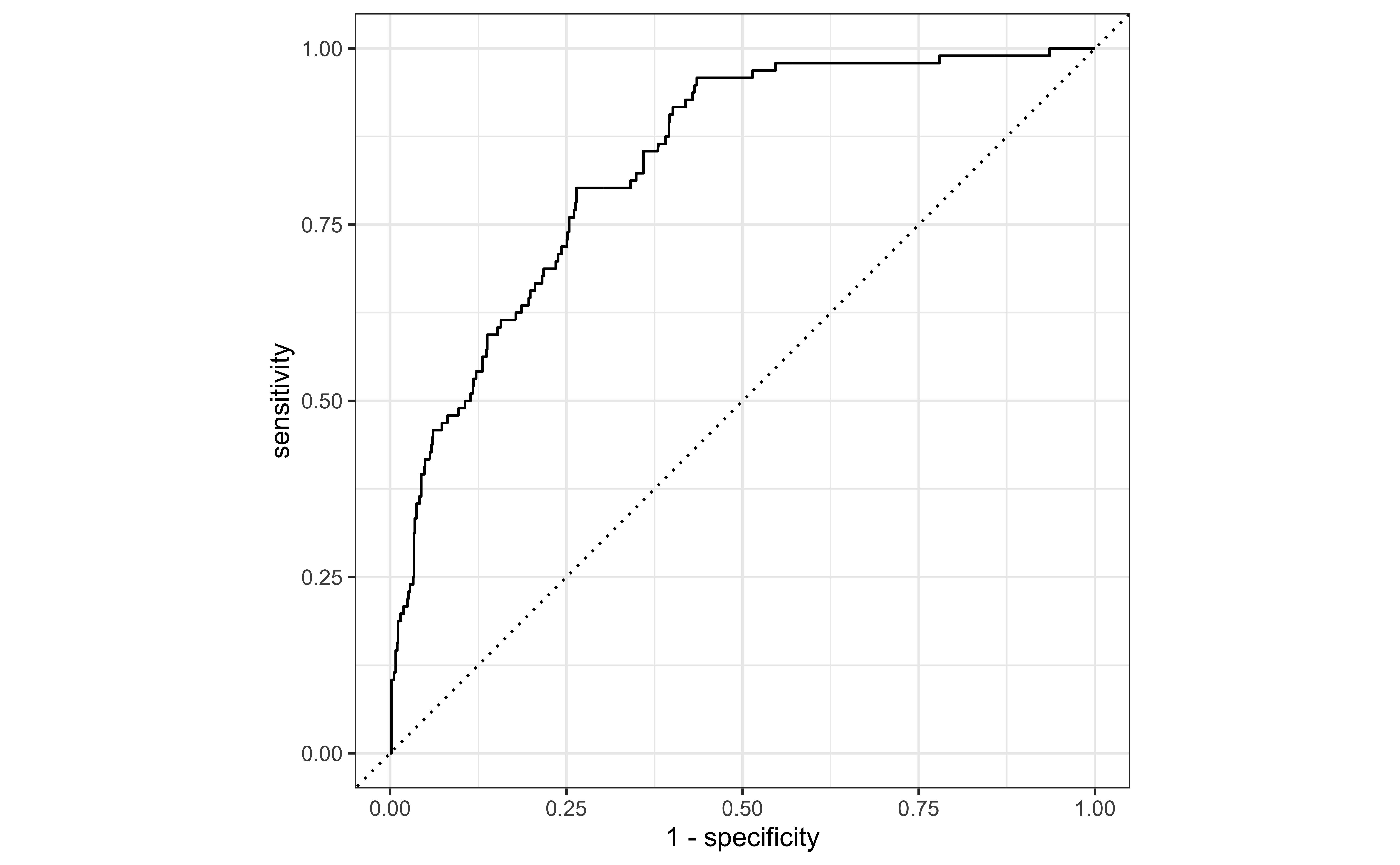
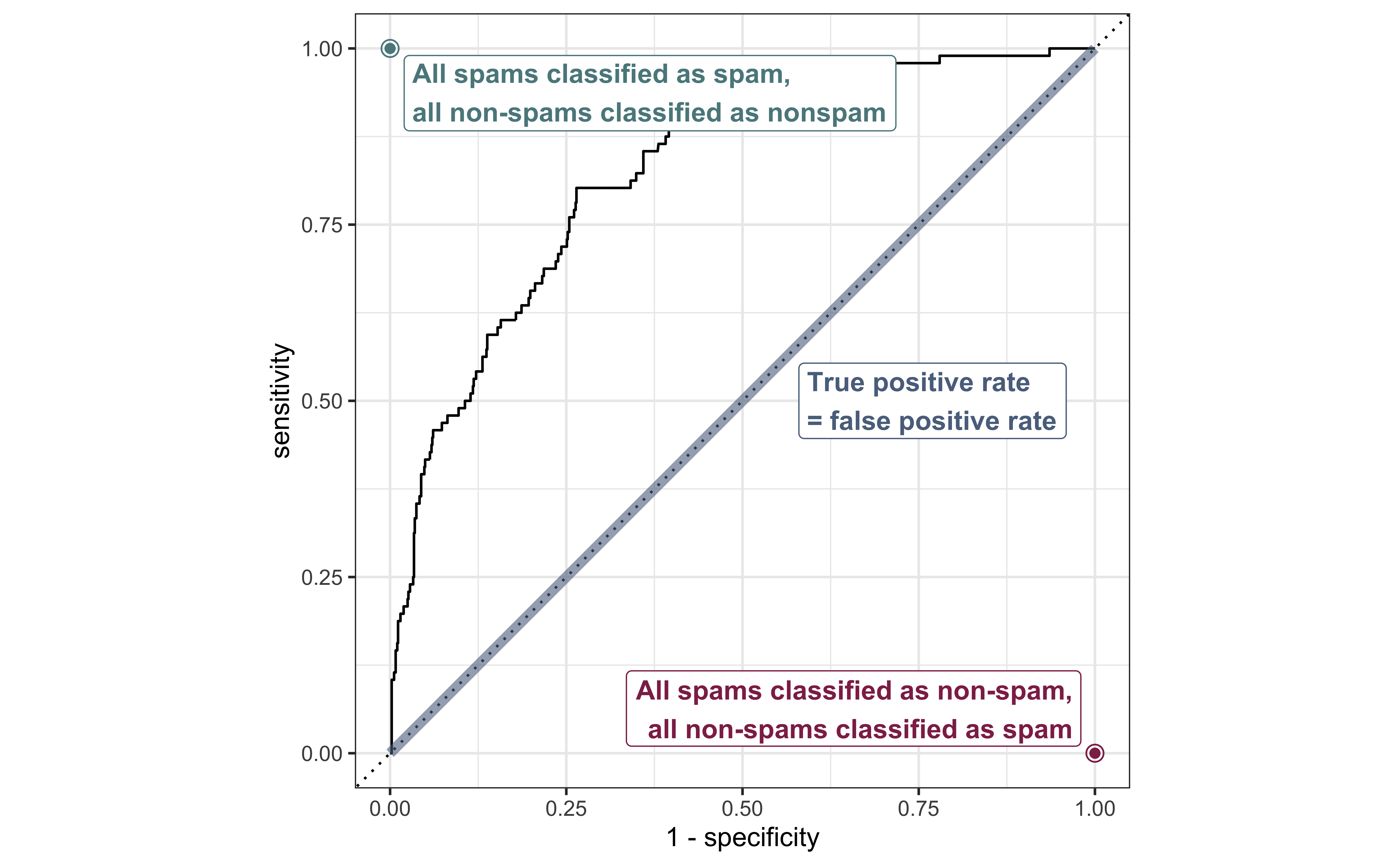
Receiver operating characteristic (ROC) curve+ plots the true positive rate (sensitivity) vs. false positive rate (1 - specificity).
ROC curve, under the hood
# A tibble: 978 × 3
    .threshold specificity sensitivity
         <dbl>       <dbl>       <dbl>
 1 -Inf            0                 1
 2    3.36e-10     0                 1
 3    2.27e- 9     0.00226           1
 4    8.69e- 7     0.00339           1
 5    9.89e- 7     0.00452           1
 6    1.43e- 6     0.00565           1
 7    9.16e- 6     0.00678           1
 8    1.03e- 5     0.00791           1
 9    2.58e- 5     0.00904           1
10    3.35e- 5     0.0102            1
# … with 968 more rows
ROC curve
Evaluate the performance: AUC
# A tibble: 1 × 3
  .metric .estimator .estimate
  <chr>   <chr>          <dbl>
1 roc_auc binary         0.836
The area under the curve (AUC) can be used to assess how well the logistic model fits the data
AUC=0.5: model is a very bad fit (no better than a coin flip)
AUC close to 1: model is a good fit
Make decisions
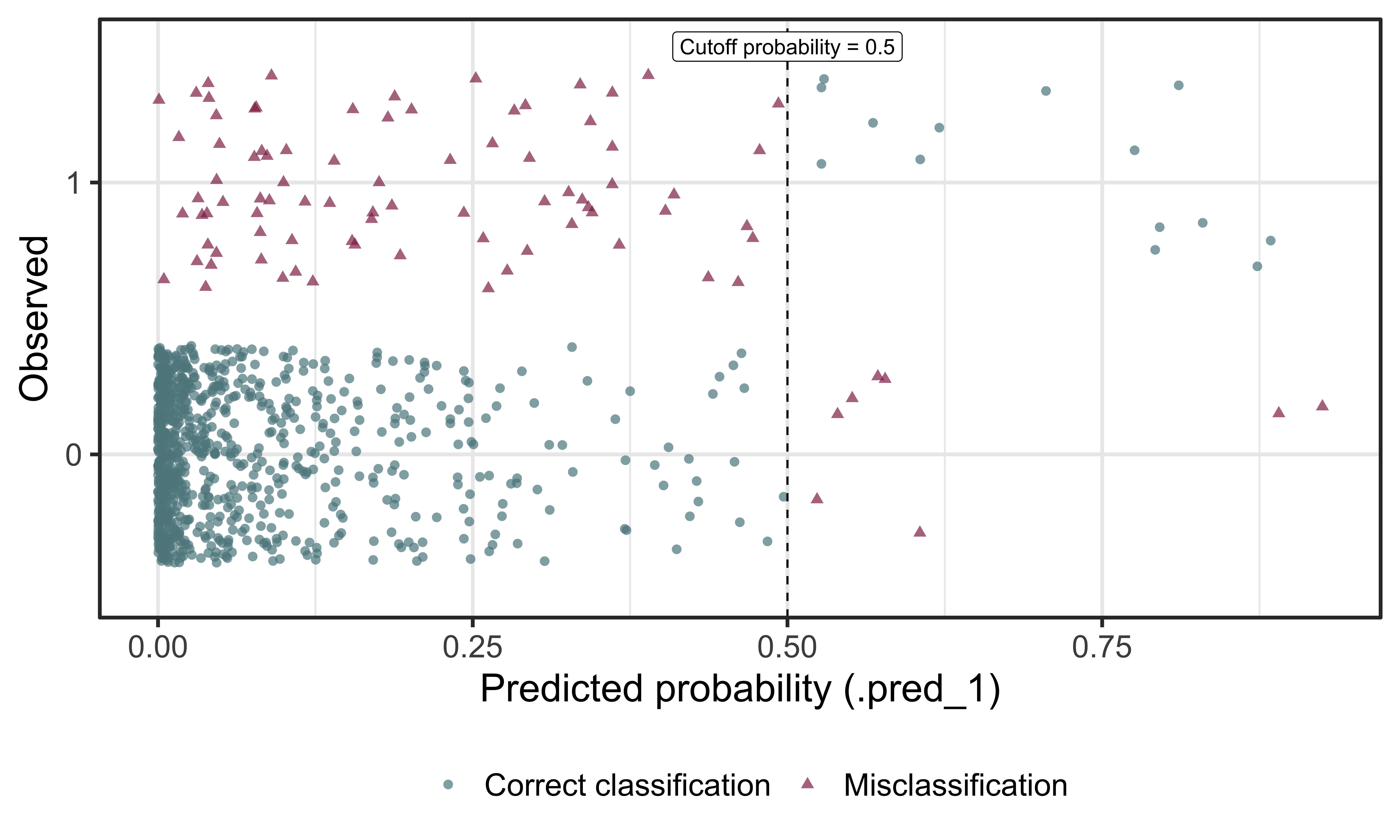
Cutoff probability: 0.5
Suppose we decide to label an email as spam if the model predicts the probability of spam to be more than 0.5.
| Email is not spam | Email is spam | |
|---|---|---|
| Email classified as not spam | 877 | 82 |
| Email classified as spam | 8 | 14 |
cutoff_prob <- 0.5
email_pred |>
  mutate(
    spam_pred = as_factor(if_else(.pred_1 >= cutoff_prob, 1, 0)),
    spam      = if_else(spam == 1, "Email is spam", "Email is not spam"),
    spam_pred = if_else(spam_pred == 1, "Email classified as spam", "Email classified as not spam")
    ) |>
  count(spam_pred, spam) |>
  pivot_wider(names_from = spam, values_from = n) |>
  kable(col.names = c("", "Email is not spam", "Email is spam"))
Confusion matrix
Cross-tabulation of observed and predicted classes:
Classification
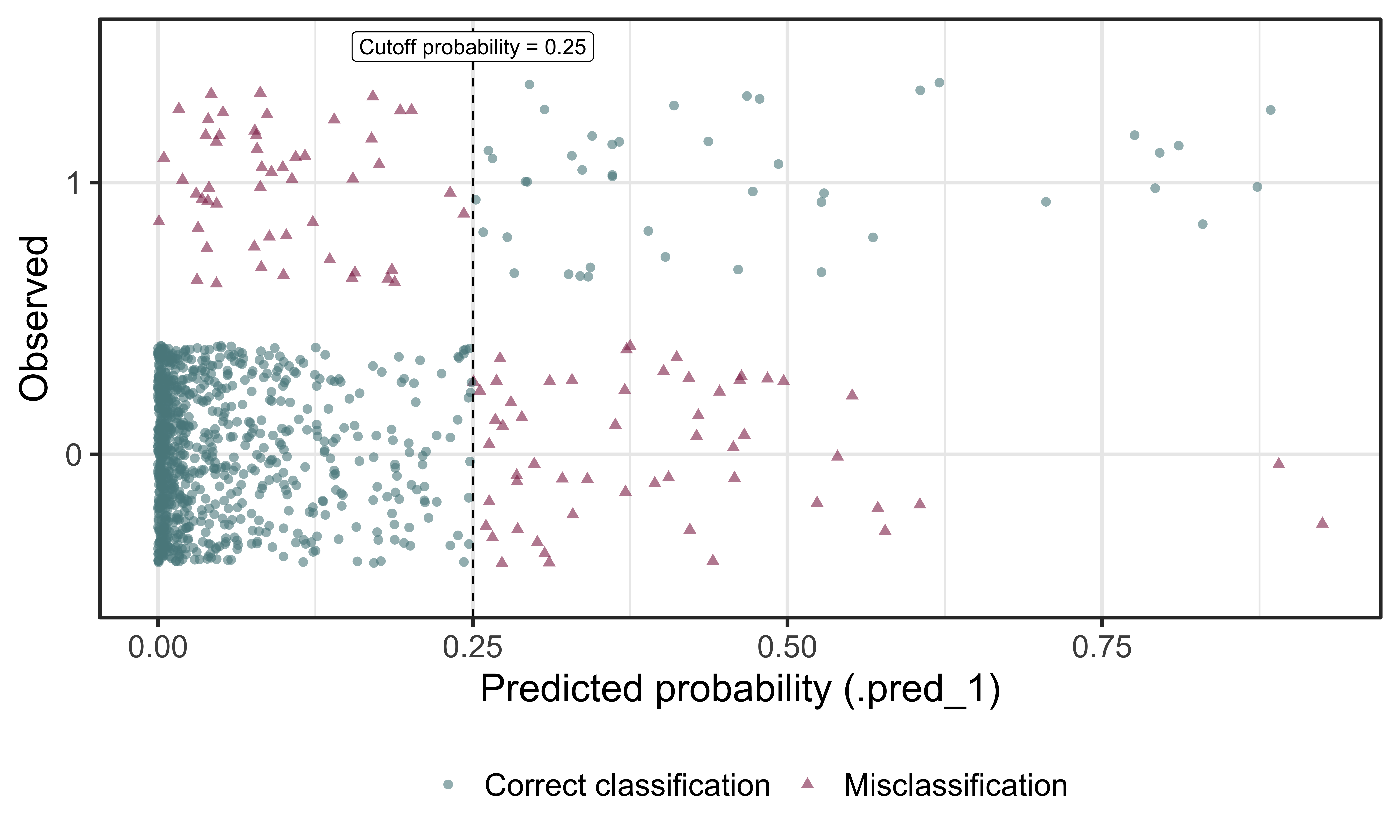
Cutoff probability: 0.25
Suppose we decide to label an email as spam if the model predicts the probability of spam to be more than 0.25.
| Email is not spam | Email is spam | |
|---|---|---|
| Email classified as not spam | 830 | 52 |
| Email classified as spam | 55 | 44 |
cutoff_prob <- 0.25
email_pred |>
  mutate(
    spam_pred = as_factor(if_else(.pred_1 >= cutoff_prob, 1, 0)),
    spam      = if_else(spam == 1, "Email is spam", "Email is not spam"),
    spam_pred = if_else(spam_pred == 1, "Email classified as spam", "Email classified as not spam")
    ) |>
  count(spam_pred, spam) |>
  pivot_wider(names_from = spam, values_from = n) |>
  kable(col.names = c("", "Email is not spam", "Email is spam"))
Classification
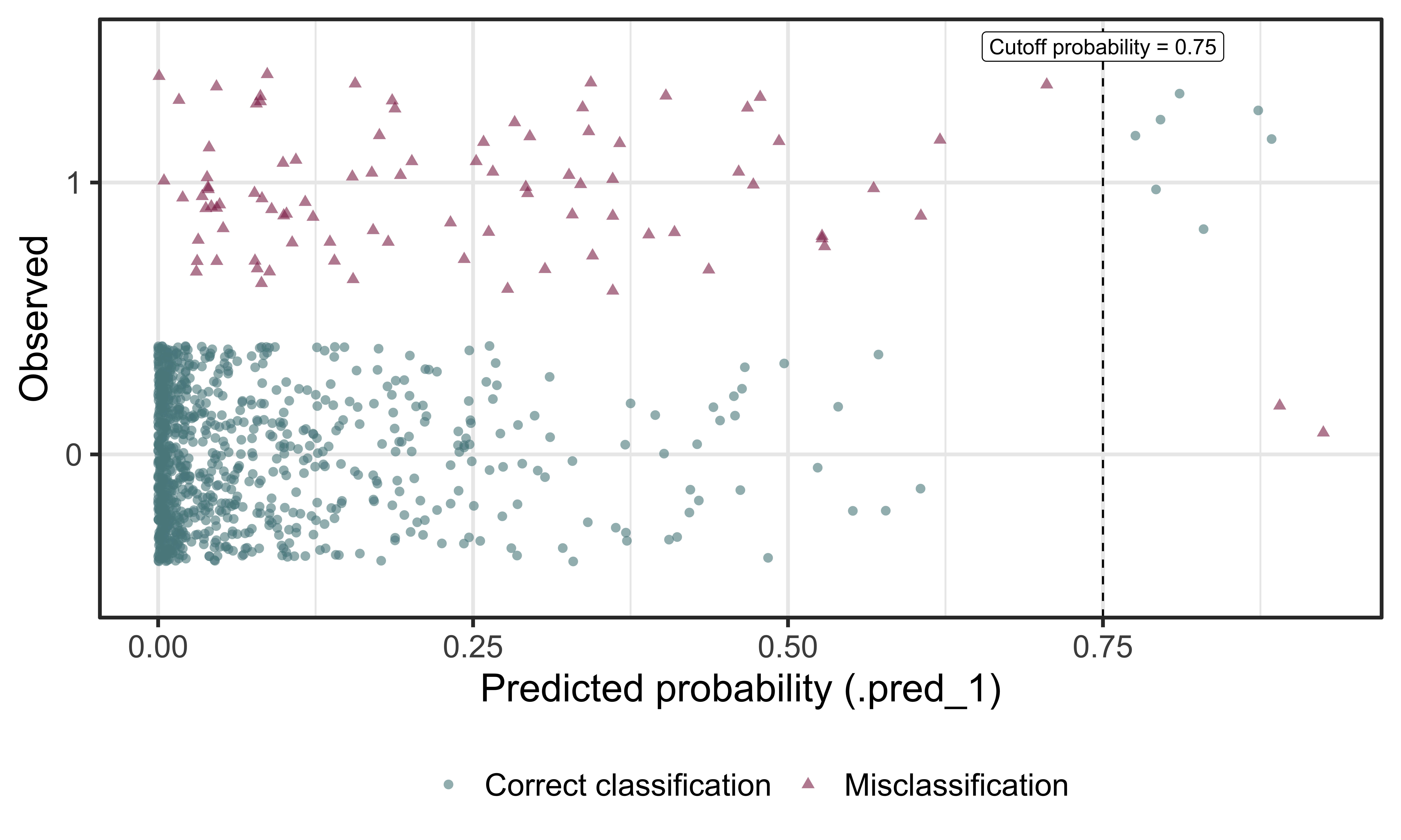
Cutoff probability: 0.75
Suppose we decide to label an email as spam if the model predicts the probability of spam to be more than 0.75.
| Email is not spam | Email is spam | |
|---|---|---|
| Email classified as not spam | 883 | 89 |
| Email classified as spam | 2 | 7 |
cutoff_prob <- 0.75
email_pred |>
  mutate(
    spam_pred = as_factor(if_else(.pred_1 >= cutoff_prob, 1, 0)),
    spam      = if_else(spam == 1, "Email is spam", "Email is not spam"),
    spam_pred = if_else(spam_pred == 1, "Email classified as spam", "Email classified as not spam")
    ) |>
  count(spam_pred, spam) |>
  pivot_wider(names_from = spam, values_from = n) |>
  kable(col.names = c("", "Email is not spam", "Email is spam"))
Classification
Use ROC curve
Use the ROC curve to determine the best cutoff probability

# A tibble: 10 × 3
   .threshold specificity sensitivity
        <dbl>       <dbl>       <dbl>
 1     0.0769       0.736       0.792
 2     0.0770       0.736       0.781
 3     0.0780       0.737       0.781
 4     0.0785       0.737       0.771
 5     0.0786       0.738       0.771
 6     0.0787       0.739       0.771
 7     0.0789       0.739       0.760
 8     0.0802       0.740       0.760
 9     0.0802       0.741       0.760
10     0.0805       0.742       0.760