LR: Inference + conditions

Prof. Maria Tackett

Nov 16, 2022

Announcements

Due dates
- HW 04 due Mon, Nov 21, 11:59pm
- Project Round 1 submission (optional) due Tue, Nov 22, 11:59pm
- Statistics experience due Fri, Dec 09, 11:59pm
No class Monday - Click here to sign up for project meeting (optional)
- Must sign up by Sun, Nov 20 at 11:59pm
See Week 12 activities

Topics

Building predictive logistic regression models
Sensitivity and specificity
Making classification decisions

Computational setup

# load packages
library(tidyverse)
library(tidymodels)
library(openintro)
library(knitr)
library(kableExtra)  # for table embellishments
library(Stat2Data)   # for empirical logit

# set default theme and larger font size for ggplot2
ggplot2::theme_set(ggplot2::theme_bw(base_size = 20))

Data

Risk of coronary heart disease

This data set is from an ongoing cardiovascular study on residents of the town of Framingham, Massachusetts. We want to examine the relationship between various health characteristics and the risk of having heart disease.

high_risk:
- 1: High risk of having heart disease in next 10 years
- 0: Not high risk of having heart disease in next 10 years
age: Age at exam time (in years)
education: 1 = Some High School, 2 = High School or GED, 3 = Some College or Vocational School, 4 = College
currentSmoker: 0 = nonsmoker, 1 = smoker

Data prep

heart_disease <- read_csv(here::here("slides", "data/framingham.csv")) |>
  select(age, education, TenYearCHD, totChol, currentSmoker) |>
  drop_na() |>
  mutate(
    high_risk = as.factor(TenYearCHD),
    education = as.factor(education),
    currentSmoker = as.factor(currentSmoker)
  )

heart_disease

# A tibble: 4,086 × 6
     age education TenYearCHD totChol currentSmoker high_risk
   <dbl> <fct>          <dbl>   <dbl> <fct>         <fct>    
 1    39 4                  0     195 0             0        
 2    46 2                  0     250 0             0        
 3    48 1                  0     245 1             0        
 4    61 3                  1     225 1             1        
 5    46 3                  0     285 1             0        
 6    43 2                  0     228 0             0        
 7    63 1                  1     205 0             1        
 8    45 2                  0     313 1             0        
 9    52 1                  0     260 0             0        
10    43 1                  0     225 1             0        
# … with 4,076 more rows

Inference for a model

Modeling risk of coronary heart disease

Using age and education:

risk_fit <- logistic_reg() |>
  set_engine("glm") |>
  fit(high_risk ~ age + education, 
      data = heart_disease, family = "binomial")

Model output

tidy(risk_fit, conf.int = TRUE) |> 
  kable(format = "markdown", digits = 3)

term	estimate	std.error	statistic	p.value	conf.low	conf.high
(Intercept)	-5.508	0.311	-17.692	0.000	-6.125	-4.904
age	0.076	0.006	13.648	0.000	0.065	0.087
education2	-0.245	0.113	-2.172	0.030	-0.469	-0.026
education3	-0.236	0.135	-1.753	0.080	-0.504	0.024
education4	-0.024	0.150	-0.161	0.872	-0.323	0.264

\[ \small{\log\Big(\frac{\hat{\pi}}{1-\hat{\pi}}\Big) = -5.508 + 0.076 ~ \text{age} - 0.245 ~ \text{ed2} - 0.236 ~ \text{ed3} - 0.024 ~ \text{ed4}} \]

Hypothesis test for \(\beta_j\)

Hypotheses: \(H_0: \beta_j = 0 \hspace{2mm} \text{ vs } \hspace{2mm} H_a: \beta_j \neq 0\)

Test Statistic: \[z = \frac{\hat{\beta}_j - 0}{SE_{\hat{\beta}_j}}\]

P-value: \(P(|Z| > |z|)\), where \(Z \sim N(0, 1)\), the Standard Normal distribution

Confidence interval for \(\beta_j\)

We can calculate the C% confidence interval for \(\beta_j\) as the following:

\[ \Large{\hat{\beta}_j \pm z^* SE_{\hat{\beta}_j}} \]

where \(z^*\) is calculated from the \(N(0,1)\) distribution

Note

This is an interval for the change in the log-odds for every one unit increase in \(x_j\)

Interpretation in terms of the odds

The change in odds for every one unit increase in \(x_j\).

\[ \Large{e^{\hat{\beta}_j \pm z^* SE_{\hat{\beta}_j}}} \]

Interpretation: We are \(C\%\) confident that for every one unit increase in \(x_j\), the odds multiply by a factor of \(e^{\hat{\beta}_j - z^* SE_{\hat{\beta}_j}}\) to \(e^{\hat{\beta}_j + z^* SE_{\hat{\beta}_j}}\), holding all else constant.

Coefficient for `age`

term	estimate	std.error	statistic	p.value	conf.low	conf.high
(Intercept)	-5.508	0.311	-17.692	0.000	-6.125	-4.904
age	0.076	0.006	13.648	0.000	0.065	0.087
education2	-0.245	0.113	-2.172	0.030	-0.469	-0.026
education3	-0.236	0.135	-1.753	0.080	-0.504	0.024
education4	-0.024	0.150	-0.161	0.872	-0.323	0.264

Hypotheses:

\[ H_0: \beta_{age} = 0 \hspace{2mm} \text{ vs } \hspace{2mm} H_a: \beta_{age} \neq 0 \]

Coefficient for `age`

term	estimate	std.error	statistic	p.value	conf.low	conf.high
(Intercept)	-5.508	0.311	-17.692	0.000	-6.125	-4.904
age	0.076	0.006	13.648	0.000	0.065	0.087
education2	-0.245	0.113	-2.172	0.030	-0.469	-0.026
education3	-0.236	0.135	-1.753	0.080	-0.504	0.024
education4	-0.024	0.150	-0.161	0.872	-0.323	0.264

Test statistic:

\[z = \frac{0.07559 - 0}{0.00554} = 13.64 \]

Coefficient for `age`

term	estimate	std.error	statistic	p.value	conf.low	conf.high
(Intercept)	-5.508	0.311	-17.692	0.000	-6.125	-4.904
age	0.076	0.006	13.648	0.000	0.065	0.087
education2	-0.245	0.113	-2.172	0.030	-0.469	-0.026
education3	-0.236	0.135	-1.753	0.080	-0.504	0.024
education4	-0.024	0.150	-0.161	0.872	-0.323	0.264

P-value:

\[ P(|Z| > |13.64|) \approx 0 \]

2 * pnorm(13.64,lower.tail = FALSE)

[1] 2.315606e-42

Coefficient for `age`

term	estimate	std.error	statistic	p.value	conf.low	conf.high
(Intercept)	-5.508	0.311	-17.692	0.000	-6.125	-4.904
age	0.076	0.006	13.648	0.000	0.065	0.087
education2	-0.245	0.113	-2.172	0.030	-0.469	-0.026
education3	-0.236	0.135	-1.753	0.080	-0.504	0.024
education4	-0.024	0.150	-0.161	0.872	-0.323	0.264

Conclusion:

The p-value is very small, so we reject \(H_0\). The data provide sufficient evidence that age is a statistically significant predictor of whether someone is high risk of having heart disease, after accounting for education.

CI for `age`

term	estimate	std.error	statistic	p.value	conf.low	conf.high
(Intercept)	-5.508	0.311	-17.692	0.000	-6.125	-4.904
age	0.076	0.006	13.648	0.000	0.065	0.087
education2	-0.245	0.113	-2.172	0.030	-0.469	-0.026
education3	-0.236	0.135	-1.753	0.080	-0.504	0.024
education4	-0.024	0.150	-0.161	0.872	-0.323	0.264

Interpret the 95% confidence interval for age in terms of the odds of being high risk for heart disease.

Comparing models

Log likelihood

\[ \log L = \sum\limits_{i=1}^n[y_i \log(\hat{\pi}_i) + (1 - y_i)\log(1 - \hat{\pi}_i)] \]

Measure of how well the model fits the data
Higher values of \(\log L\) are better
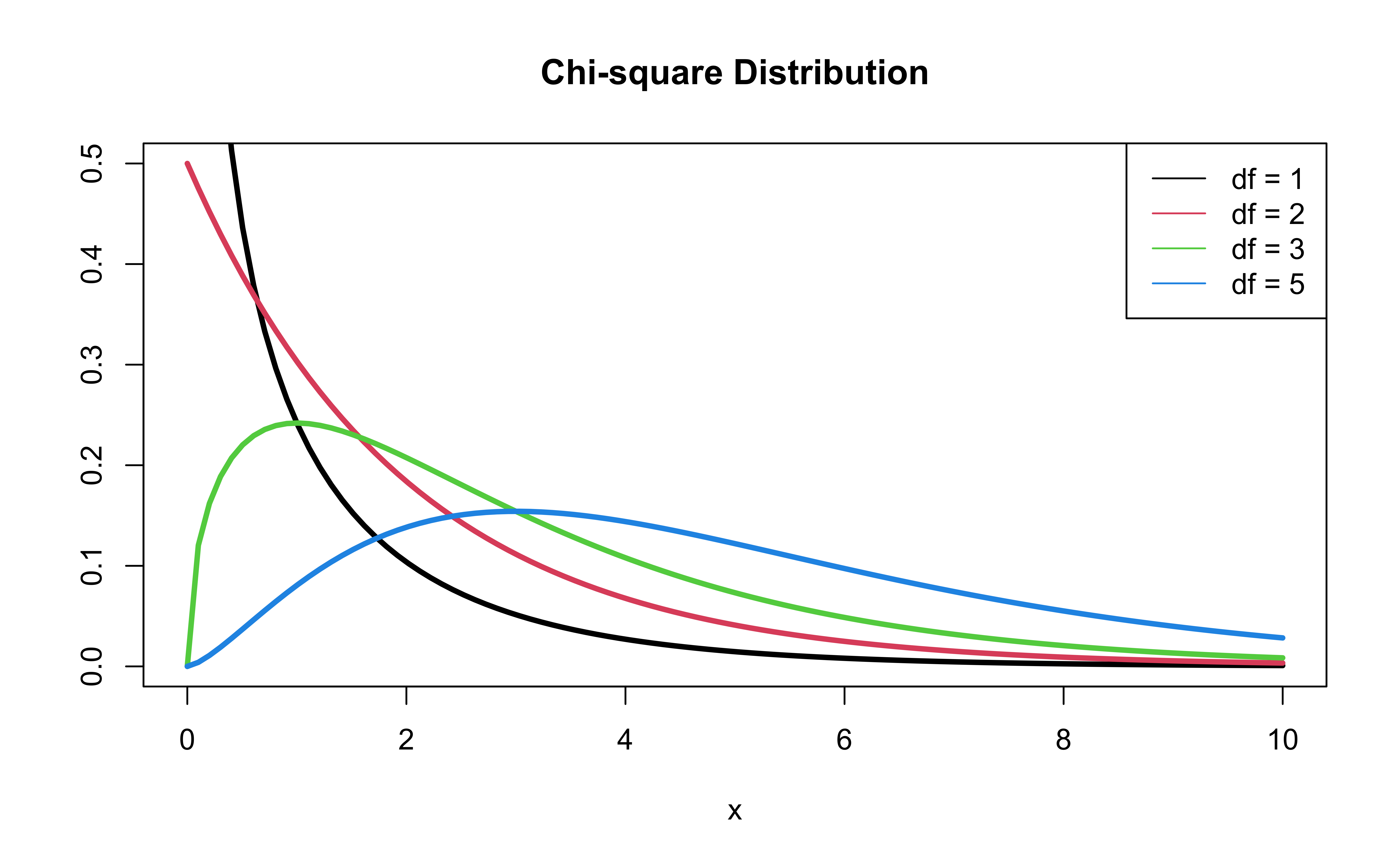
Deviance = \(-2 \log L\)
- \(-2 \log L\) follows a \(\chi^2\) distribution with \(n - p - 1\) degrees of freedom

Model with age and education

Should we add currentSmoker to this model?

term	estimate	std.error	statistic	p.value	conf.low	conf.high
(Intercept)	-5.508	0.311	-17.692	0.000	-6.125	-4.904
age	0.076	0.006	13.648	0.000	0.065	0.087
education2	-0.245	0.113	-2.172	0.030	-0.469	-0.026
education3	-0.236	0.135	-1.753	0.080	-0.504	0.024
education4	-0.024	0.150	-0.161	0.872	-0.323	0.264

Should we add `currentSmoker` to the model?

First model, reduced:

risk_fit_reduced <- logistic_reg() |>
  set_engine("glm") |>
  fit(high_risk ~ age + education, 
      data = heart_disease, family = "binomial")

Second model, full:

risk_fit_full <- logistic_reg() |>
  set_engine("glm") |>
  fit(high_risk ~ age + education + currentSmoker, 
      data = heart_disease, family = "binomial")

Model selection

Use AIC or BIC for model selection

\[ \begin{align} &AIC = - 2 * \log L - \color{purple}{n\log(n)}+ 2(p +1)\\[5pt] &BIC =- 2 * \log L - \color{purple}{n\log(n)} + log(n)\times(p+1) \end{align} \]

AIC from the `glance()` function

Let’s look at the AIC for the model that includes age, education, and currentSmoker

glance(risk_fit_full)$AIC

[1] 3233.901

Calculating AIC

- 2 * glance(risk_fit_full)$logLik + 2 * (5 + 1)

[1] 3233.901

Comparing the models using AIC

Let’s compare the full and reduced models using AIC.

glance(risk_fit_reduced)$AIC

[1] 3254.187

glance(risk_fit_full)$AIC

[1] 3233.901

Based on AIC, which model would you choose?

Comparing the models using BIC

Let’s compare the full and reduced models using BIC

glance(risk_fit_reduced)$BIC

[1] 3285.764

glance(risk_fit_full)$BIC

[1] 3271.793

Based on BIC, which model would you choose?

Conditions

The model

Let’s predict high_risk from age, total cholesterol, and whether the patient is a current smoker:

risk_fit <- logistic_reg() |>
  set_engine("glm") |>
  fit(high_risk ~ age + totChol + currentSmoker, 
      data = heart_disease, family = "binomial")

tidy(risk_fit, conf.int = TRUE) |> 
  kable(digits = 3)

term	estimate	std.error	statistic	p.value	conf.low	conf.high
(Intercept)	-6.673	0.378	-17.647	0.000	-7.423	-5.940
age	0.082	0.006	14.344	0.000	0.071	0.094
totChol	0.002	0.001	1.940	0.052	0.000	0.004
currentSmoker1	0.443	0.094	4.733	0.000	0.260	0.627

Conditions for logistic regression

Linearity: The log-odds have a linear relationship with the predictors.
Randomness: The data were obtained from a random process
Independence: The observations are independent from one another.

Empirical logit

The empirical logit is the log of the observed odds:

\[ \text{logit}(\hat{p}) = \log\Big(\frac{\hat{p}}{1 - \hat{p}}\Big) = \log\Big(\frac{\# \text{Yes}}{\# \text{No}}\Big) \]

Calculating empirical logit (categorical predictor)

If the predictor is categorical, we can calculate the empirical logit for each level of the predictor.

heart_disease |>
  count(currentSmoker, high_risk) |>
  group_by(currentSmoker) |>
  mutate(prop = n/sum(n)) |>
  filter(high_risk == "1") |>
  mutate(emp_logit = log(prop/(1-prop)))

# A tibble: 2 × 5
# Groups:   currentSmoker [2]
  currentSmoker high_risk     n  prop emp_logit
  <fct>         <fct>     <int> <dbl>     <dbl>
1 0             1           301 0.145     -1.77
2 1             1           318 0.158     -1.67

Calculating empirical logit (quantitative predictor)

Divide the range of the predictor into intervals with approximately equal number of cases. (If you have enough observations, use 5 - 10 intervals.)
Calculate the mean value of the predictor in each interval.
Compute the empirical logit for each interval.

Then, create a plot of the empirical logit versus the mean value of the predictor in each interval.

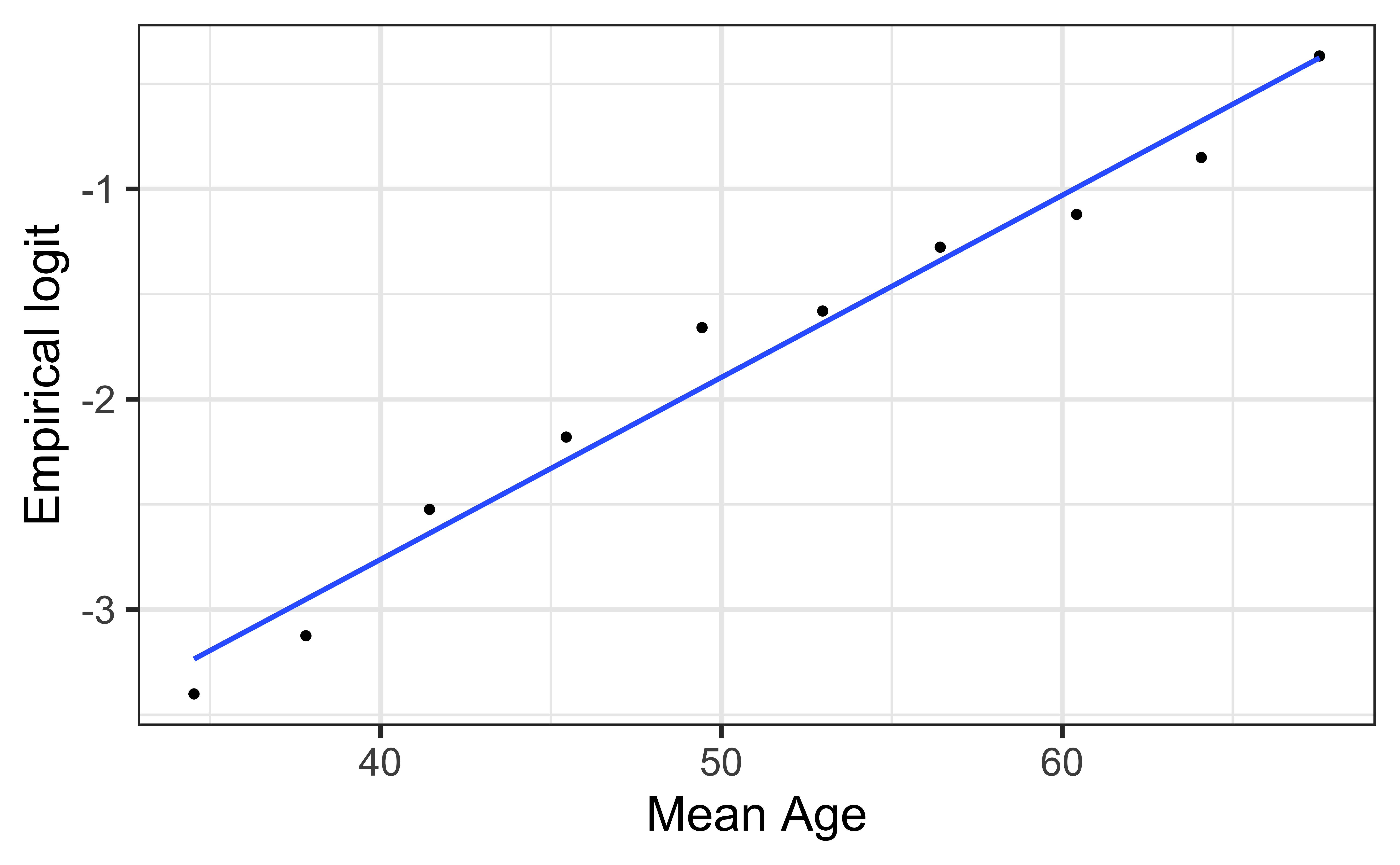
Empirical logit plot in R (quantitative predictor)

Created using dplyr and ggplot functions.

Empirical logit plot in R (quantitative predictor)

Created using dplyr and ggplot functions.

heart_disease |> 
  mutate(age_bin = cut_interval(age, n = 10)) |>
  group_by(age_bin) |>
  mutate(mean_age = mean(age)) |>
  count(mean_age, high_risk) |>
  mutate(prop = n/sum(n)) |>
  filter(high_risk == "1") |>
  mutate(emp_logit = log(prop/(1-prop))) |>
  ggplot(aes(x = mean_age, y = emp_logit)) + 
  geom_point() + 
  geom_smooth(method = "lm", se = FALSE) +
  labs(x = "Mean Age", 
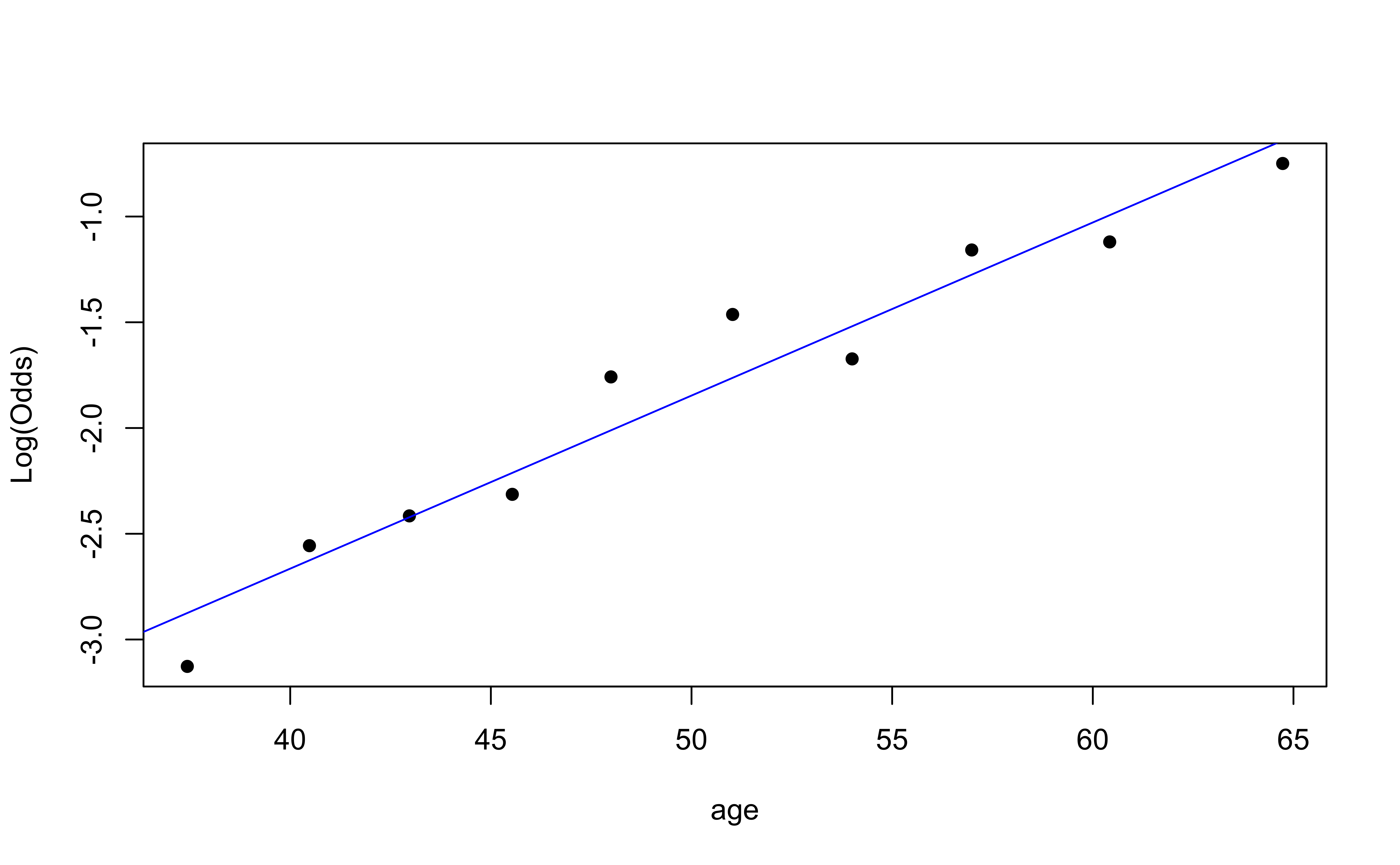
       y = "Empirical logit")

Empirical logit plot in R (quantitative predictor)

Using the emplogitplot1 function from the Stat2Data R package

emplogitplot1(high_risk ~ age, 
              data = heart_disease, 
              ngroups = 10)

Empirical logit plot in R (interactions)

Using the emplogitplot2 function from the Stat2Data R package

emplogitplot2(high_risk ~ age + currentSmoker, data = heart_disease, 
              ngroups = 10, 
              putlegend = "bottomright")

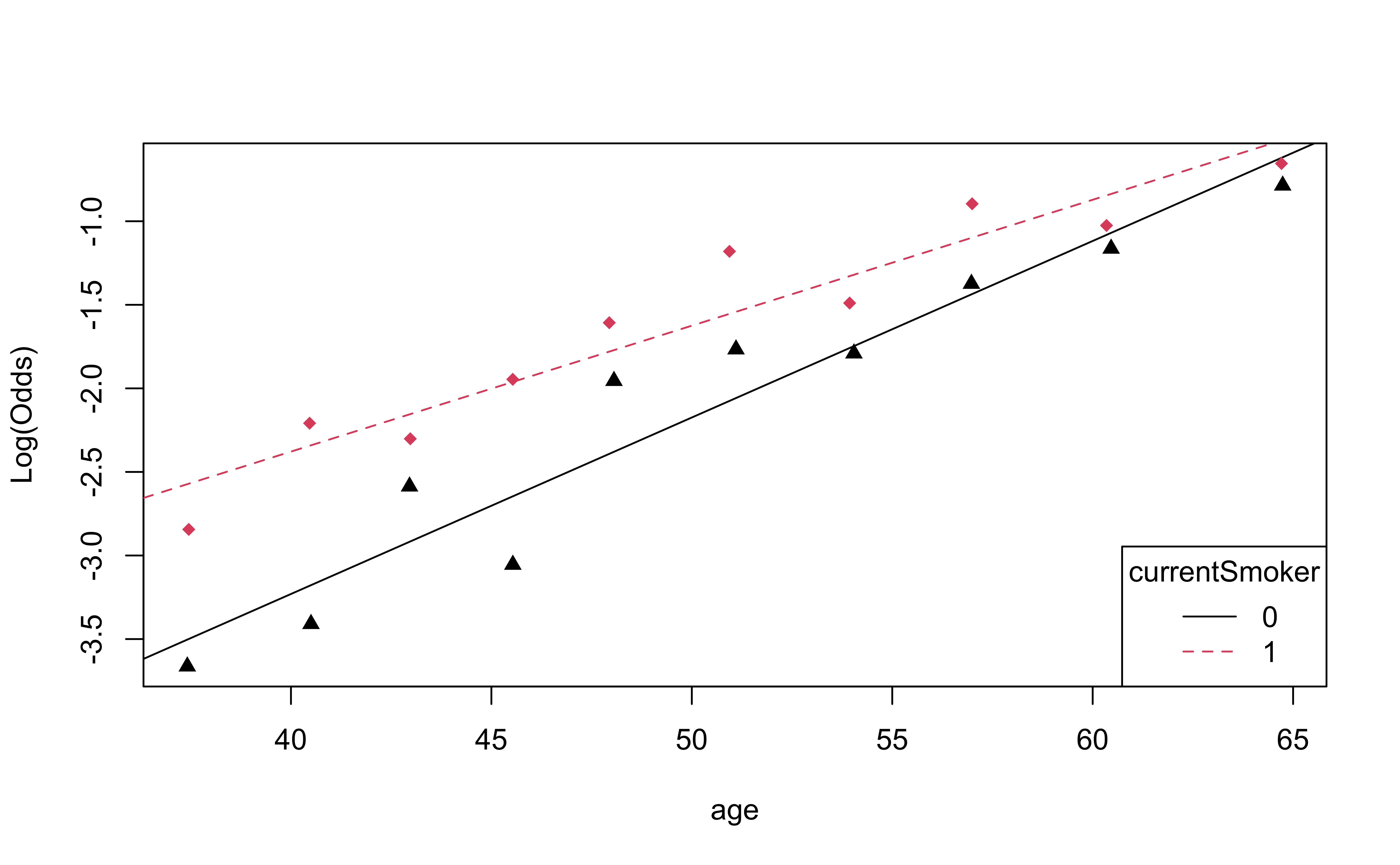
Checking linearity

emplogitplot1(high_risk ~ age, 
              data = heart_disease, 
              ngroups = 10)

emplogitplot1(high_risk ~ totChol, 
              data = heart_disease, 
              ngroups = 10)

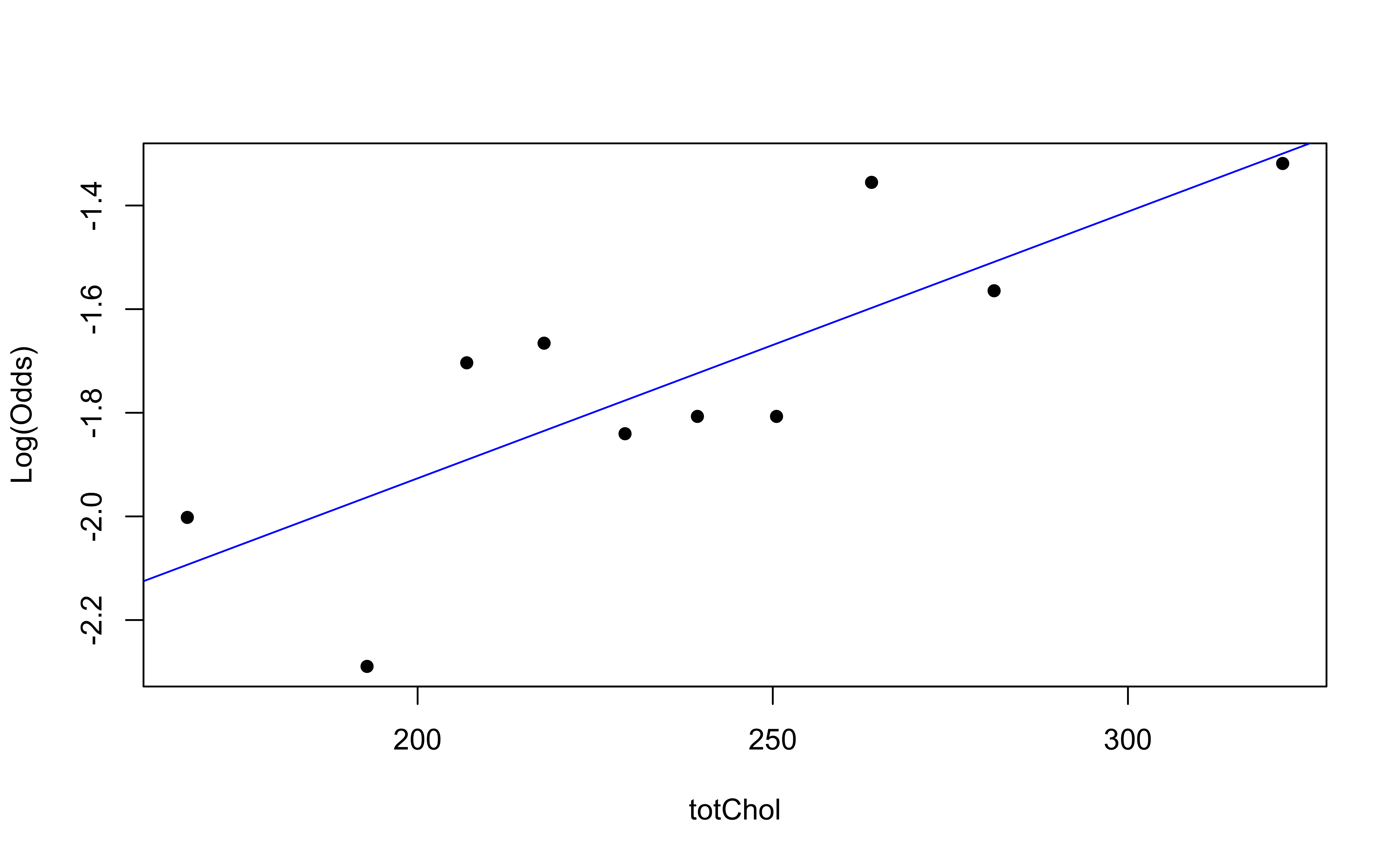
✅ The linearity condition is satisfied. There is a linear relationship between the empirical logit and the predictor variables.

Checking randomness

We can check the randomness condition based on the context of the data and how the observations were collected.

Was the sample randomly selected?
If the sample was not randomly selected, ask whether there is reason to believe the observations in the sample differ systematically from the population of interest.

✅ The randomness condition is satisfied. We do not have reason to believe that the participants in this study differ systematically from adults in the U.S. in regards to health characteristics and risk of heart disease.

Checking independence

We can check the independence condition based on the context of the data and how the observations were collected.
Independence is most often violated if the data were collected over time or there is a strong spatial relationship between the observations.

✅ The independence condition is satisfied. It is reasonable to conclude that the participants’ health characteristics are independent of one another.

Comparing nested models using the drop-in-deviance test (optional)

Comparing nested models

Suppose there are two models:
- Reduced Model includes predictors \(x_1, \ldots, x_q\)
- Full Model includes predictors \(x_1, \ldots, x_q, x_{q+1}, \ldots, x_p\)
We want to test the hypotheses

\[ \begin{aligned} H_0&: \beta_{q+1} = \dots = \beta_p = 0 \\ H_A&: \text{ at least 1 }\beta_j \text{ is not } 0 \end{aligned} \]
To do so, we will use the Drop-in-deviance test, also known as the Nested Likelihood Ratio test

Drop-in-deviance test

Hypotheses:

\[ \begin{aligned} H_0&: \beta_{q+1} = \dots = \beta_p = 0 \\ H_A&: \text{ at least 1 }\beta_j \text{ is not } 0 \end{aligned} \]

Test Statistic: \[G = (-2 \log L_{reduced}) - (-2 \log L_{full})\]

P-value: \(P(\chi^2 > G)\), calculated using a \(\chi^2\) distribution with degrees of freedom equal to the difference in the number of parameters in the full and reduced models

\(\chi^2\) distribution

Should we add `currentSmoker` to the model?

Calculate deviance for each model:

(dev_reduced <- glance(risk_fit_reduced)$deviance)

[1] 3244.187

(dev_full <- glance(risk_fit_full)$deviance)

[1] 3221.901

Drop-in-deviance test statistic:

(test_stat <- dev_reduced - dev_full)

[1] 22.2863

Should we add `currentSmoker` to the model?

Calculate the p-value using a pchisq(), with degrees of freedom equal to the number of new model terms in the second model:

pchisq(test_stat, 1, lower.tail = FALSE)

[1] 2.348761e-06

Conclusion: The p-value is very small, so we reject \(H_0\). The data provide sufficient evidence that the coefficient of currentSmoker is not equal to 0. Therefore, we should add it to the model.

Drop-in-Deviance test in R

We can use the anova function to conduct this test
Add test = "Chisq" to conduct the drop-in-deviance test

anova(risk_fit_reduced$fit, risk_fit_full$fit, test = "Chisq") |>
  tidy() |> kable(digits = 3)

term	Resid..Df	Resid..Dev	df	Deviance	p.value
high_risk ~ age + education	4081	3244.187	NA	NA	NA
high_risk ~ age + education + currentSmoker	4080	3221.901	1	22.286	0

LR: Inference + conditions

Announcements

Topics

Computational setup

Data

Risk of coronary heart disease

Data prep

Inference for a model

Modeling risk of coronary heart disease

Model output

Hypothesis test for \(\beta_j\)

Confidence interval for \(\beta_j\)

Interpretation in terms of the odds

Coefficient for age

Coefficient for age

Coefficient for age

Coefficient for age

CI for age

Comparing models

Log likelihood

Model with age and education

Should we add currentSmoker to the model?

Model selection

AIC from the glance() function

Comparing the models using AIC

Comparing the models using BIC

Conditions

The model

Conditions for logistic regression

Empirical logit

Calculating empirical logit (categorical predictor)

Calculating empirical logit (quantitative predictor)

Empirical logit plot in R (quantitative predictor)

Empirical logit plot in R (quantitative predictor)

Empirical logit plot in R (quantitative predictor)

Empirical logit plot in R (interactions)

Checking linearity

Checking randomness

Checking independence

Comparing nested models using the drop-in-deviance test (optional)

Comparing nested models

Drop-in-deviance test

\(\chi^2\) distribution

Should we add currentSmoker to the model?

Should we add currentSmoker to the model?

Drop-in-Deviance test in R

Coefficient for `age`

Coefficient for `age`

Coefficient for `age`

Coefficient for `age`

CI for `age`

Should we add `currentSmoker` to the model?

AIC from the `glance()` function

Should we add `currentSmoker` to the model?

Should we add `currentSmoker` to the model?