SLR: Simulation-based inference

Bootstrap confidence intervals for the slope

Prof. Maria Tackett

Sep 12, 2022

Announcements

• Lab 01 due

  • TODAY, 11:59pm (Thursday labs)

  • Tuesday, 11:59pm (Friday labs)

  • Make sure all work is pushed to GitHub and the PDF is submitted on Gradescope by the deadline

• See Week 03 for this week’s activities.

Topics

• Assess model’s predictive importance using data splitting and bootstrapping

• Find range of plausible values for the slope using bootstrap confidence intervals

Computational setup

# load packages
library(tidyverse)   # for data wrangling and visualization
library(tidymodels)  # for modeling
library(usdata)      # for the county_2019 dataset
library(openintro)   # for Duke Forest dataset
library(scales)      # for pretty axis labels
library(glue)        # for constructing character strings
library(knitr)       # for neatly formatted tables
library(kableExtra)  # also for neatly formatted tablesf


# set default theme and larger font size for ggplot2
ggplot2::theme_set(ggplot2::theme_bw(base_size = 16))

Recap of last class

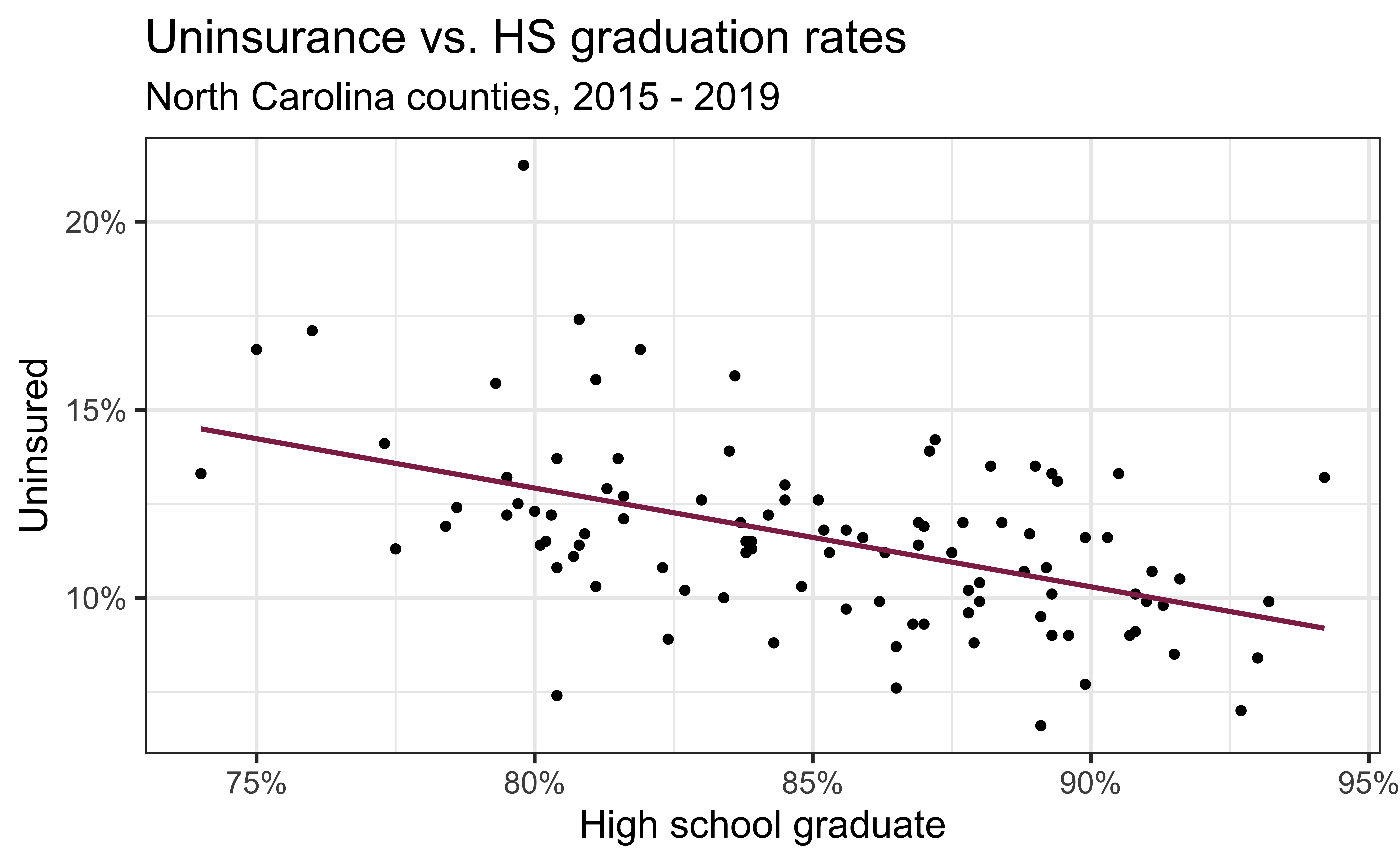
Uninsurance vs. HS graduation rates

Code

ggplot(county_2019_nc, aes(x = hs_grad, y = uninsured)) +
  geom_point() +
  geom_smooth(method = "lm", se = FALSE, color = "#8F2D56") +
  scale_x_continuous(labels = label_percent(scale = 1, accuracy = 1)) +
  scale_y_continuous(labels = label_percent(scale = 1, accuracy = 1)) +
  labs(
    x = "High school graduate", y = "Uninsured",
    title = "Uninsurance vs. HS graduation rates",
    subtitle = "North Carolina counties, 2015 - 2019"
  )

Fitting the model

nc_fit <- linear_reg() |>
  set_engine("lm") |>
  fit(uninsured ~ hs_grad, data = county_2019_nc)

tidy(nc_fit)

# A tibble: 2 × 5
  term        estimate std.error statistic  p.value
  <chr>          <dbl>     <dbl>     <dbl>    <dbl>
1 (Intercept)   33.9      3.99        8.50 2.12e-13
2 hs_grad       -0.262    0.0468     -5.61 1.88e- 7

Augmenting the data

With augment() to add columns for predicted values (.fitted), residuals (.resid), etc.:

nc_aug <- augment(nc_fit$fit)
nc_aug

# A tibble: 100 × 8
   uninsured hs_grad .fitted  .resid   .hat .sigma    .cooksd .std.resid
       <dbl>   <dbl>   <dbl>   <dbl>  <dbl>  <dbl>      <dbl>      <dbl>
 1      11.2    86.3   11.3  -0.0633 0.0107   2.10 0.00000501    -0.0305
 2       8.9    82.4   12.3  -3.39   0.0138   2.07 0.0186        -1.63  
 3      11.3    77.5   13.6  -2.27   0.0393   2.09 0.0252        -1.11  
 4      11.1    80.7   12.7  -1.63   0.0199   2.09 0.00633       -0.790 
 5      12.6    85.1   11.6   1.02   0.0100   2.10 0.00122        0.492 
 6      15.9    83.6   12.0   3.93   0.0112   2.06 0.0203         1.89  
 7      12      87.7   10.9   1.10   0.0133   2.10 0.00191        0.532 
 8      11.9    78.4   13.3  -1.44   0.0328   2.09 0.00830       -0.700 
 9      12.9    81.3   12.6   0.324  0.0174   2.10 0.000218       0.157 
10       9.8    91.3    9.95 -0.151  0.0291   2.10 0.0000806     -0.0734
# … with 90 more rows

Statistics for model evaluation

• R-squared, \(R^2\) : Percentage of variability in the outcome explained by the regression model (in the context of SLR, the predictor)

  \[ R^2 = Cor(x,y)^2 = Cor(y, \hat{y})^2 \]

• Root mean square error, RMSE: A measure of the average error (average difference between observed and predicted values of the outcome)

  \[ RMSE = \sqrt{\frac{\sum_{i = 1}^n (y_i - \hat{y}_i)^2}{n}} \]

Obtaining \(R^2\) and RMSE

Use rsq() and rmse(), respectively

rsq(nc_aug, truth = uninsured, estimate = .fitted)

# A tibble: 1 × 3
  .metric .estimator .estimate
  <chr>   <chr>          <dbl>
1 rsq     standard       0.243

rmse(nc_aug, truth = uninsured, estimate = .fitted)

# A tibble: 1 × 3
  .metric .estimator .estimate
  <chr>   <chr>          <dbl>
1 rmse    standard        2.07

Purpose of model evaluation

• \(R^2\) tells us how our model is doing to predict the data we already have
• But generally we are interested in prediction for a new observation, not for one that is already in our sample, i.e. out-of-sample prediction
• We have a couple ways of simulating out-of-sample prediction before actually getting new data to evaluate the performance of our models

Splitting data

Spending our data

• There are several steps to create a useful model: parameter estimation, model selection, performance assessment, etc.
• Doing all of this on the entire data we have available leaves us with no other data to assess our choices
• We can allocate specific subsets of data for different tasks, as opposed to allocating the largest possible amount to the model parameter estimation only (which is what we’ve done so far)

Simulation: data splitting

• Take a random sample of 10% of the data and set aside (testing data)
• Fit a model on the remaining 90% of the data (training data)
• Use the coefficients from this model to make predictions for the testing data
• Repeat 10 times

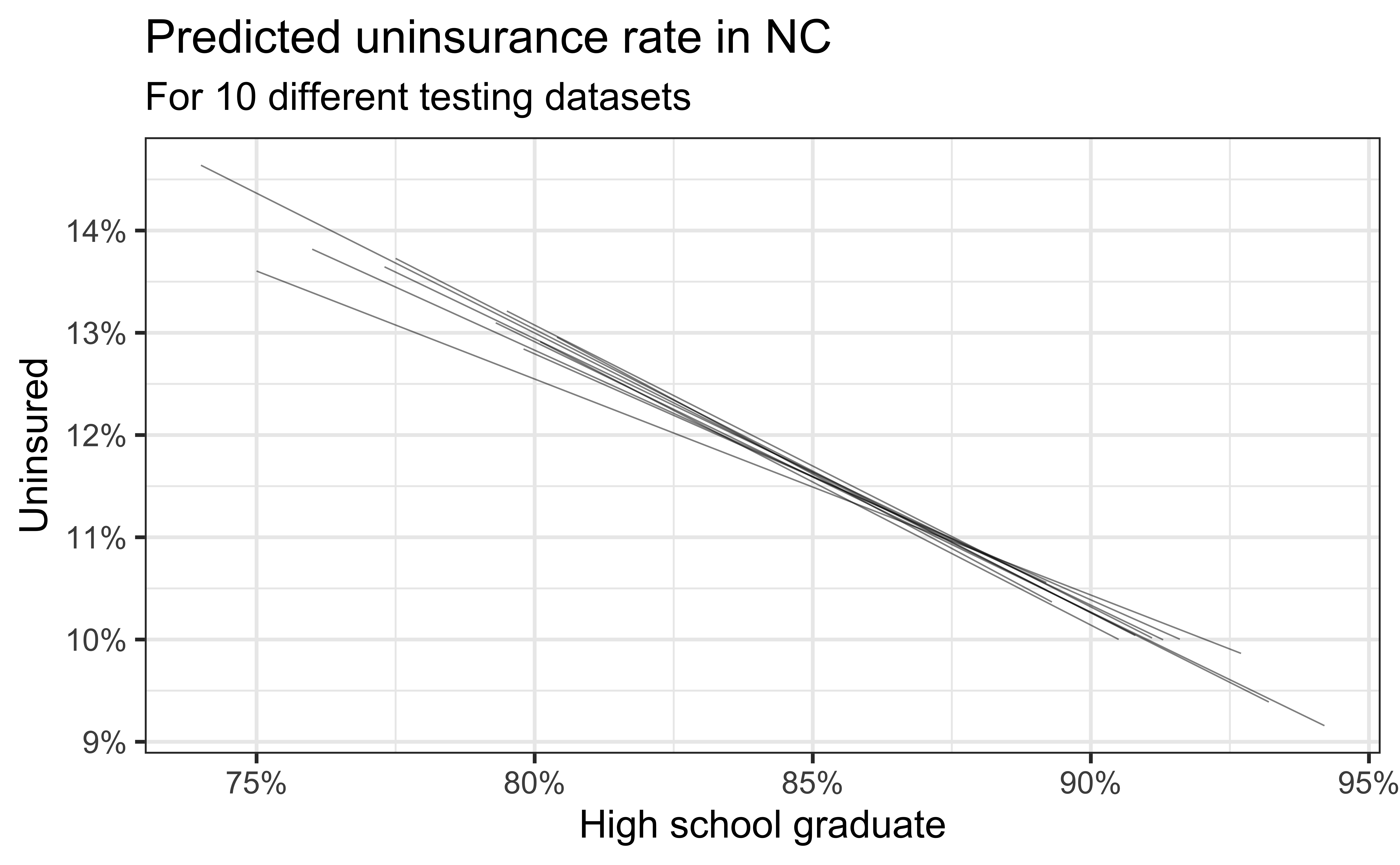
Predictive performance

• How consistent are the predictions for different testing datasets?
• How consistent are the predictions for counties with high school graduation rates in the middle of the plot vs. in the edges?

Bootstrapping

Bootstrapping our data

• The idea behind bootstrapping is that if a given observation exists in a sample, there may be more like it in the population
• With bootstrapping, we simulate resampling from the population by resampling from the sample we observed
• Bootstrap samples are the sampled with replacement from the original sample and same size as the original sample
  • For example, if our sample consists of the observations {A, B, C}, bootstrap samples could be {A, A, B}, {A, C, A}, {B, C, C}, {A, B, C}, etc.

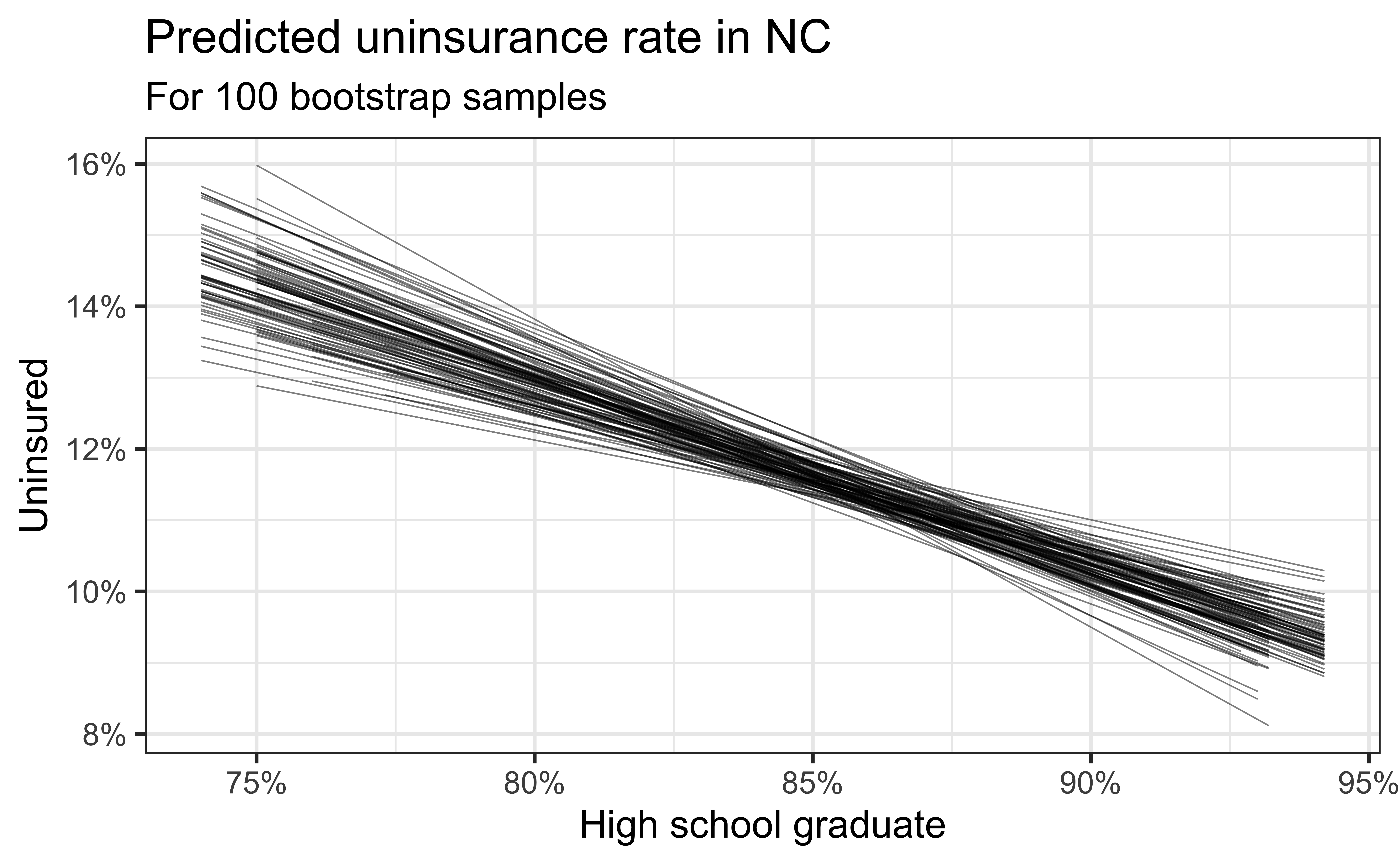
Simulation: bootstrapping

• Take a bootstrap sample – sample with replacement from the original data, same size as the original data
• Fit model to the sample and make predictions for that sample
• Repeat many times

Predictive performance

• How consistent are the predictions for different bootstrap datasets?
• How consistent are the predictions for counties with high school graduation rates in the middle of the plot vs. in the edges?

Recap

• Motivated the importance of model evaluation

• Described how \(R^2\) and RMSE are used to evaluate models

• Assessed model’s predictive importance using data splitting and bootstrapping

Simulation-based inference

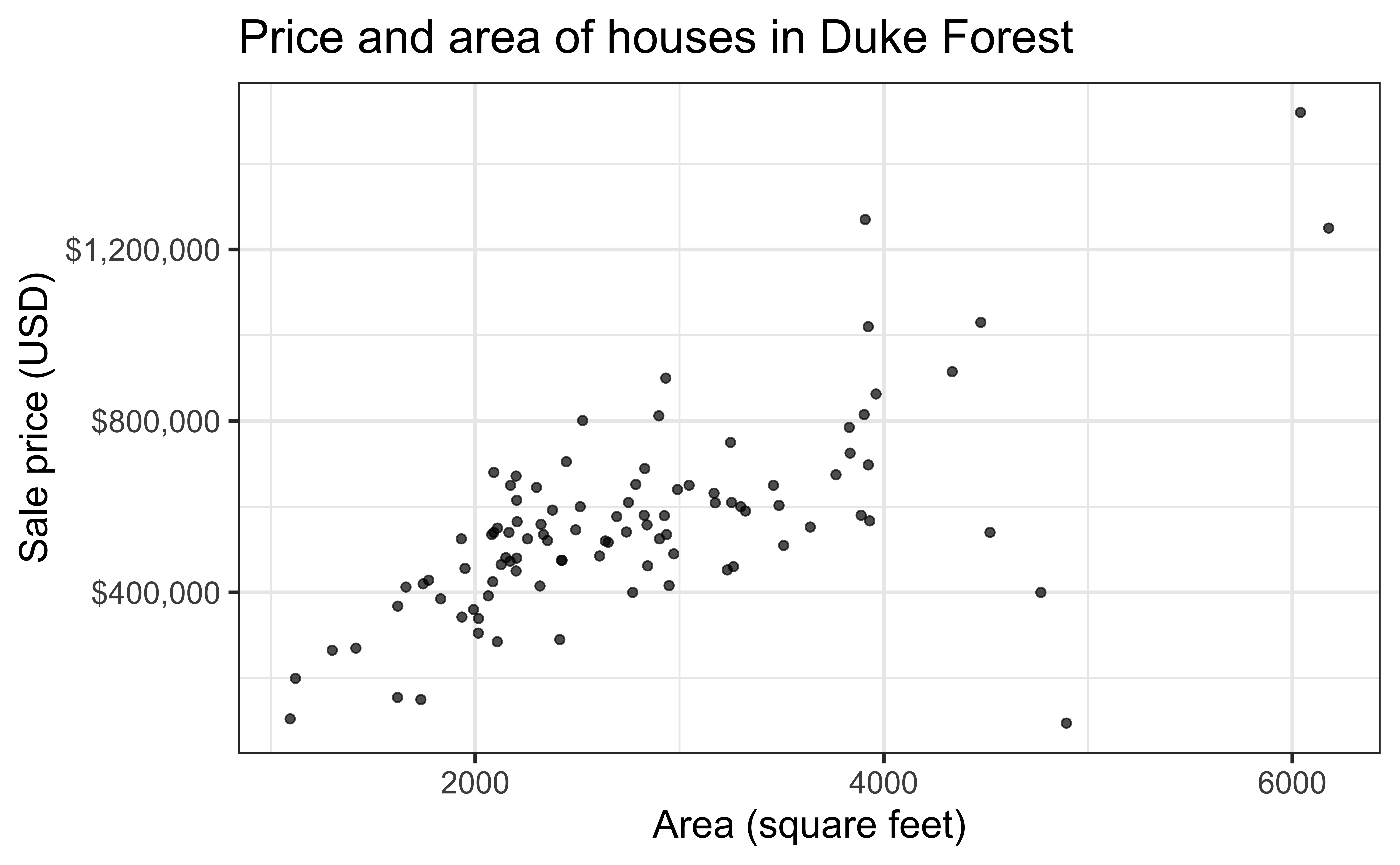
Data: Houses in Duke Forest

• Data on houses that were sold in the Duke Forest neighborhood of Durham, NC around November 2020
• Scraped from Zillow
• Source: openintro::duke_forest

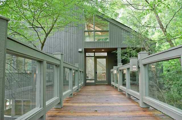
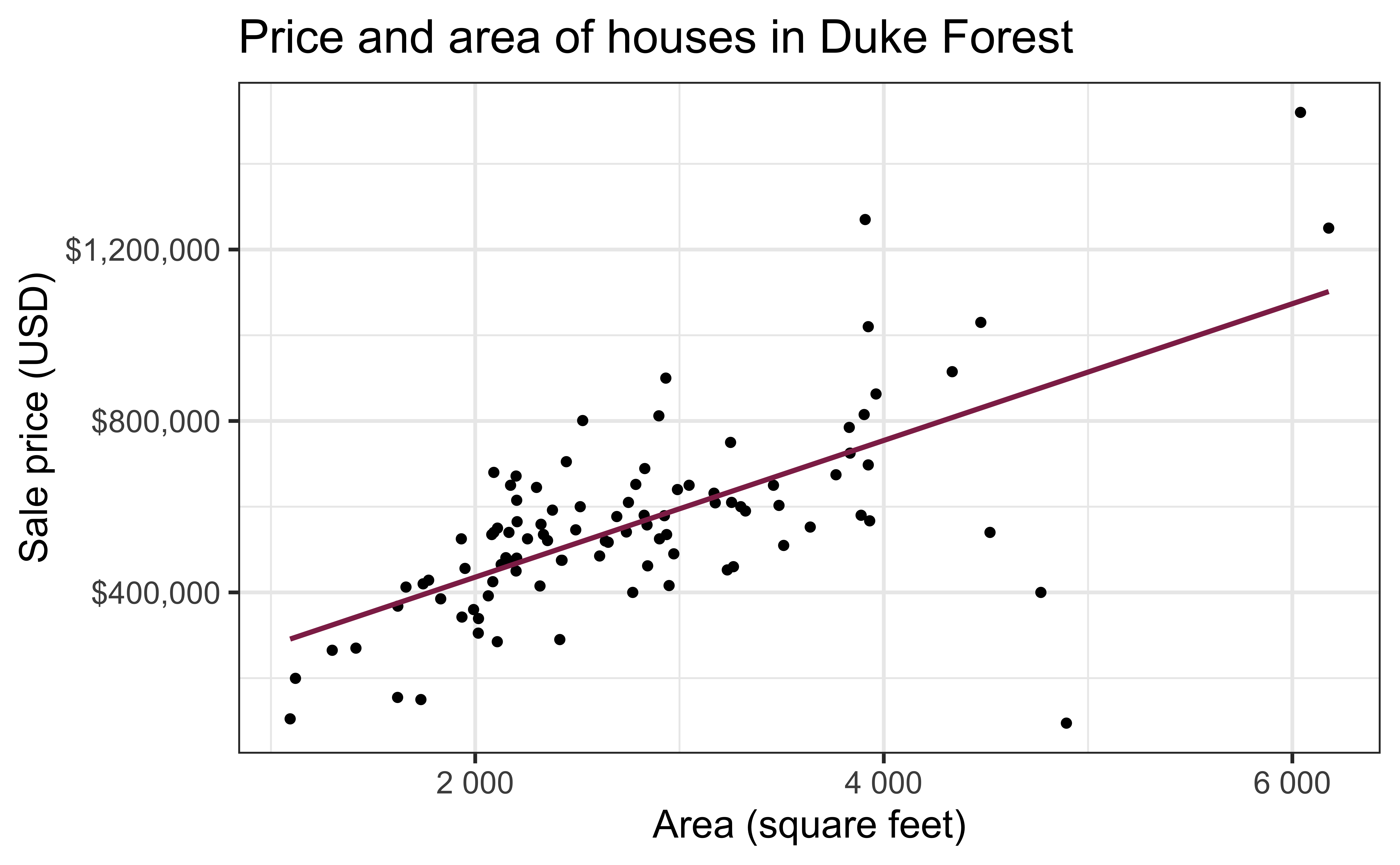
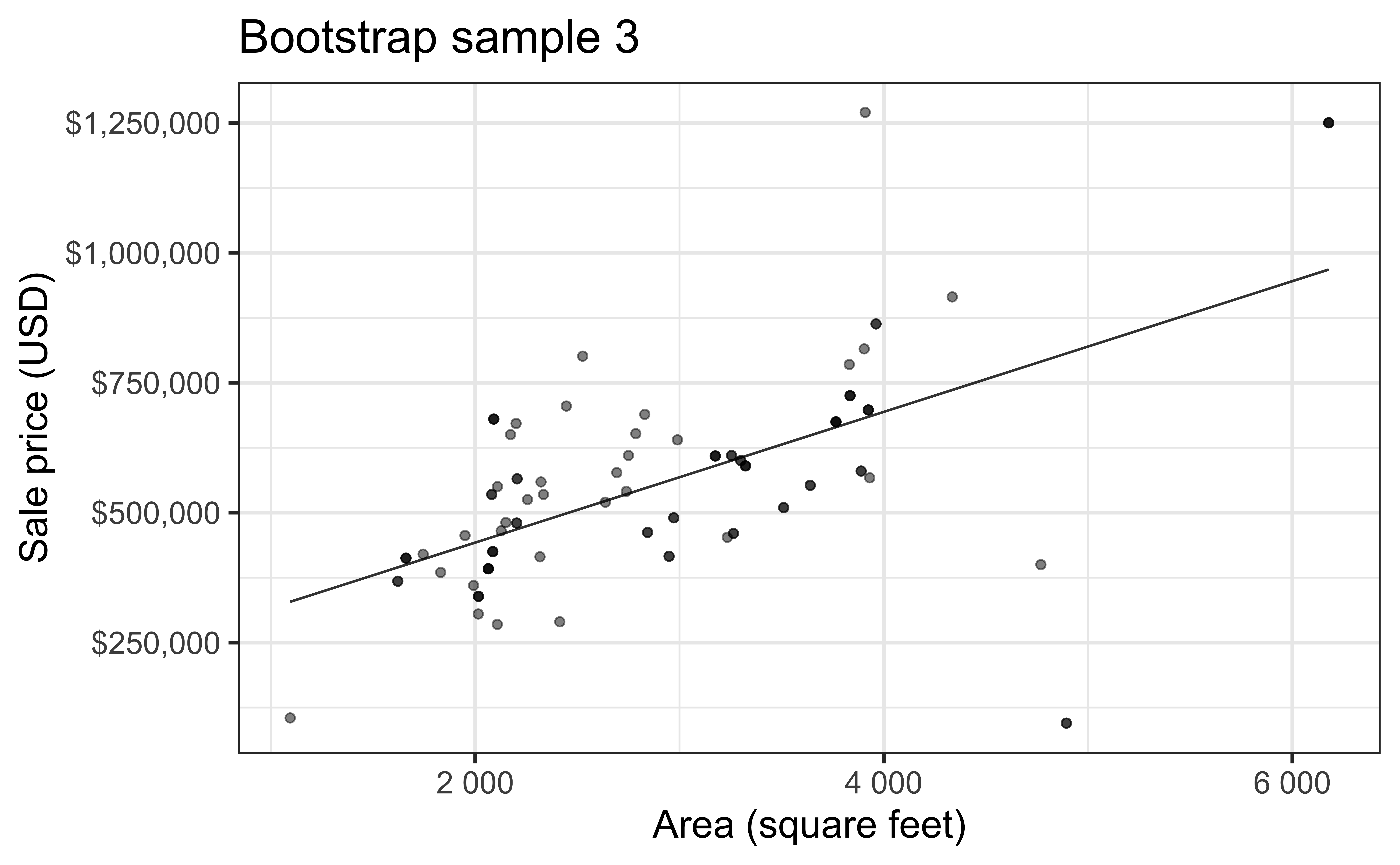
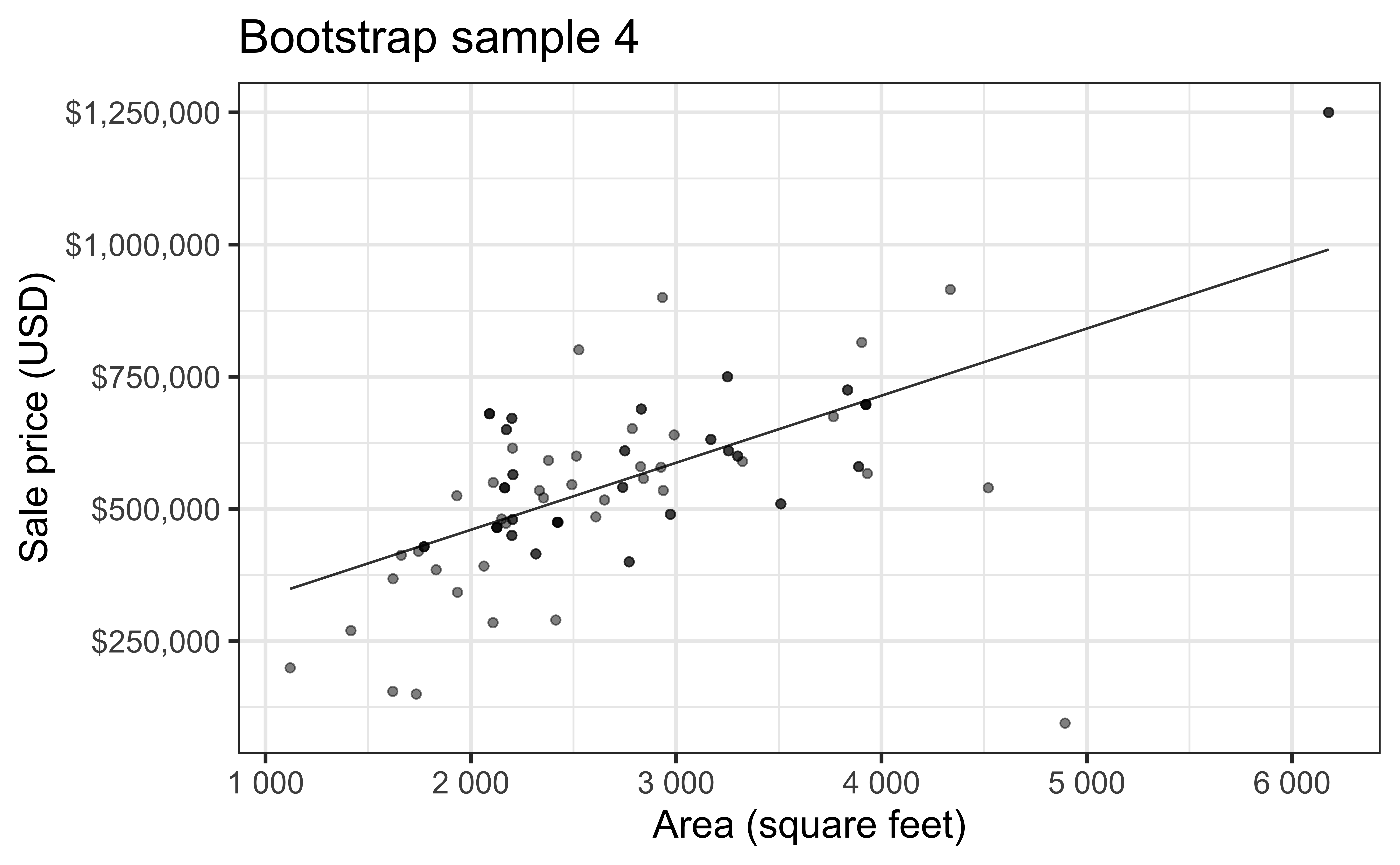
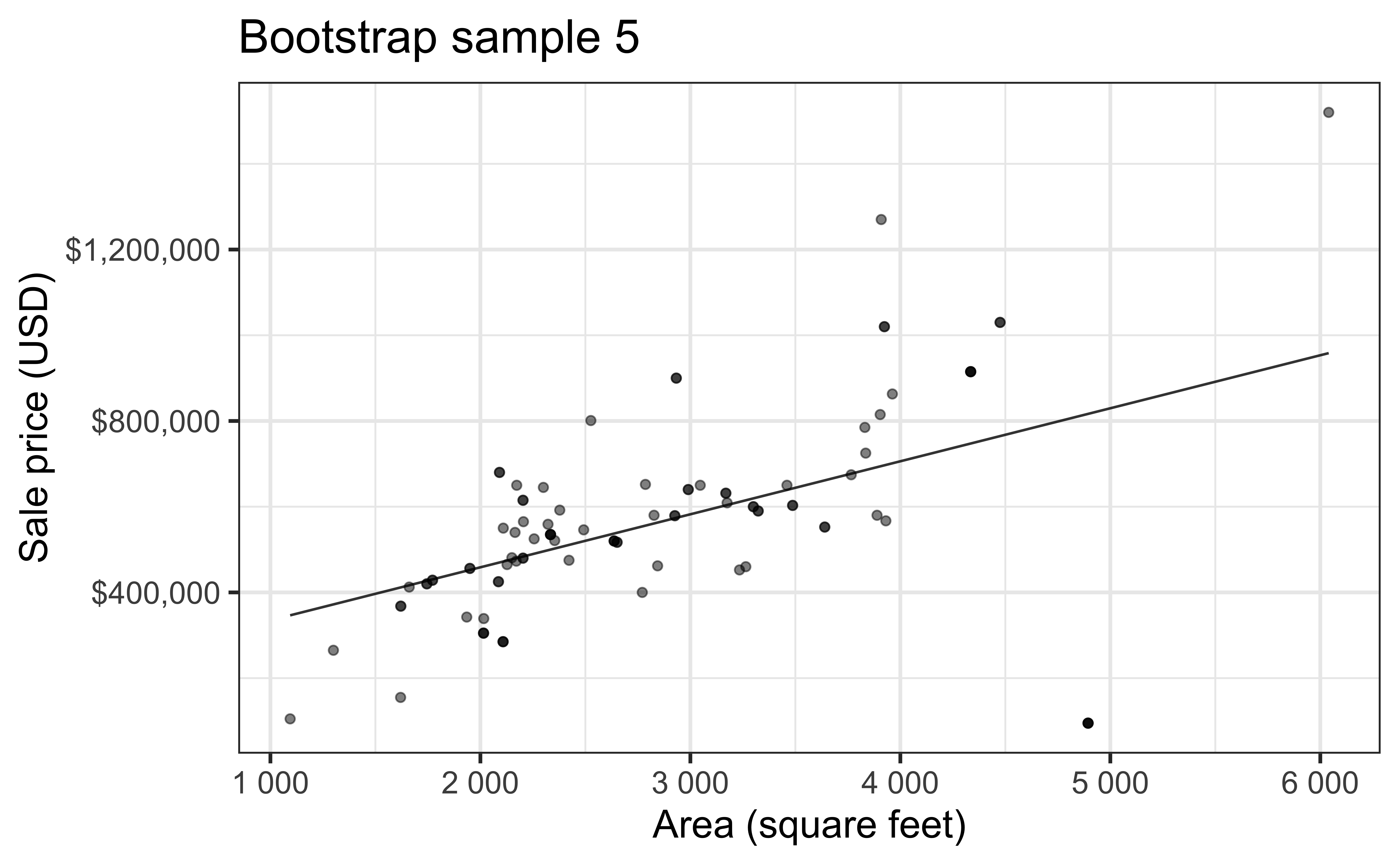
Goal: Use the area (in square feet) to understand variability in the price of houses in Duke Forest.

Exploratory data analysis

Code

ggplot(duke_forest, aes(x = area, y = price)) +
  geom_point(alpha = 0.7) +
  labs(
    x = "Area (square feet)",
    y = "Sale price (USD)",
    title = "Price and area of houses in Duke Forest"
  ) +
  scale_y_continuous(labels = label_dollar()) 

Modeling

df_fit <- linear_reg() |>
  set_engine("lm") |>
  fit(price ~ area, data = duke_forest)

tidy(df_fit) |>
  kable(digits = 2) #neatly format table to 2 digits

term	estimate	std.error	statistic	p.value
(Intercept)	116652.33	53302.46	2.19	0.03
area	159.48	18.17	8.78	0.00

• Intercept: Duke Forest houses that are 0 square feet are expected to sell, on average, for $116,652.
• Slope: For each additional square foot, the model predicts the sale price of Duke Forest houses to be higher, on average, by $159.

From sample to population

For each additional square foot, the model predicts the sale price of Duke Forest houses to be higher, on average, by $159.

• This estimate is valid for the single sample of 98 houses.
• But what if we’re not interested quantifying the relationship between the size and price of a house in this single sample?
• What if we want to say something about the relationship between these variables for all houses in Duke Forest?

Statistical inference

• Statistical inference provide methods and tools so we can use the single observed sample to make valid statements (inferences) about the population it comes from

• For our inferences to be valid, the sample should be random and representative of the population we’re interested in

Inference for simple linear regression

• Calculate a confidence interval for the slope, \(\beta_1\)

• Conduct a hypothesis test for the slope,\(\beta_1\)

Confidence interval for the slope

Confidence interval

• A plausible range of values for a population parameter is called a confidence interval
• Using only a single point estimate is like fishing in a murky lake with a spear, and using a confidence interval is like fishing with a net
  • We can throw a spear where we saw a fish but we will probably miss, if we toss a net in that area, we have a good chance of catching the fish
  • Similarly, if we report a point estimate, we probably will not hit the exact population parameter, but if we report a range of plausible values we have a good shot at capturing the parameter

Confidence interval for the slope

A confidence interval will allow us to make a statement like “For each additional square foot, the model predicts the sale price of Duke Forest houses to be higher, on average, by $159, plus or minus X dollars.”

• Should X be $10? $100? $1000?

• If we were to take another sample of 98 would we expect the slope calculated based on that sample to be exactly $159? Off by $10? $100? $1000?

• The answer depends on how variable (from one sample to another sample) the sample statistic (the slope) is

• We need a way to quantify the variability of the sample statistic

Quantify the variability of the slope

for estimation

• Two approaches:
  1. Via simulation (what we’ll do today)
  2. Via mathematical models (what we’ll do in the next class)
• Bootstrapping to quantify the variability of the slope for the purpose of estimation:
  • Bootstrap new samples from the original sample
  • Fit models to each of the samples and estimate the slope
  • Use features of the distribution of the bootstrapped slopes to construct a confidence interval

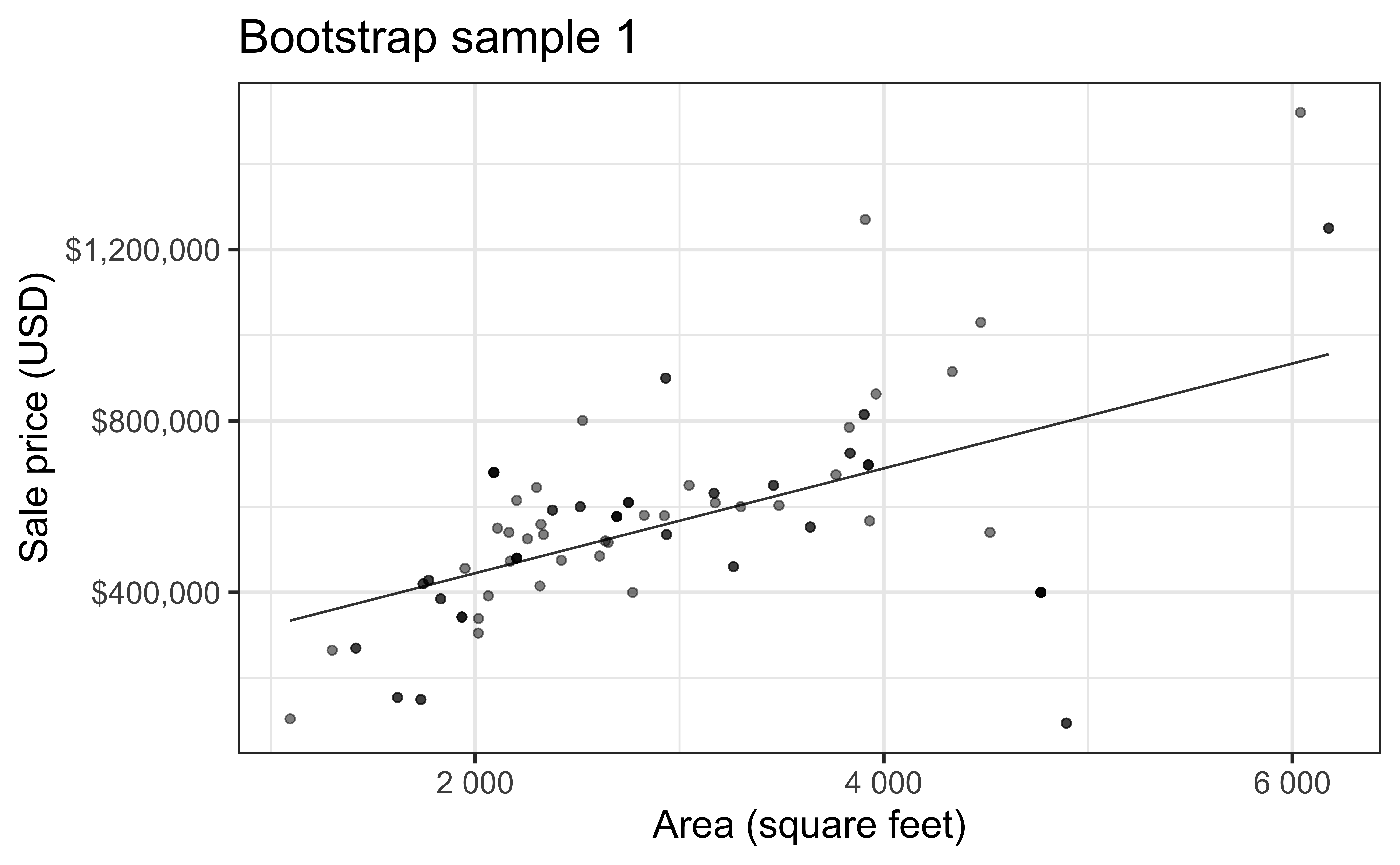
Bootstrap sample 1

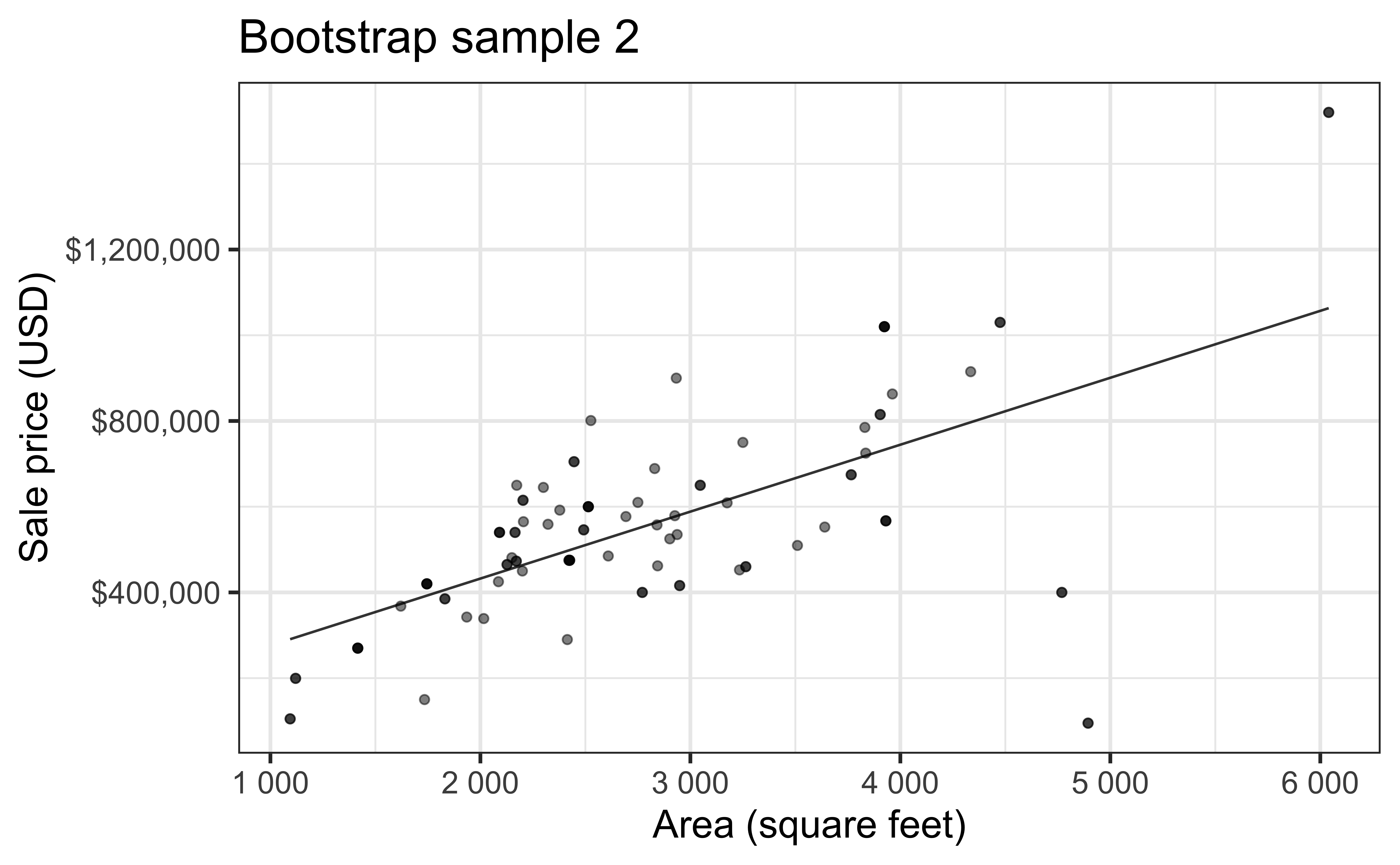
Bootstrap sample 2

Bootstrap sample 3

Bootstrap sample 4

Bootstrap sample 5

so on and so forth…

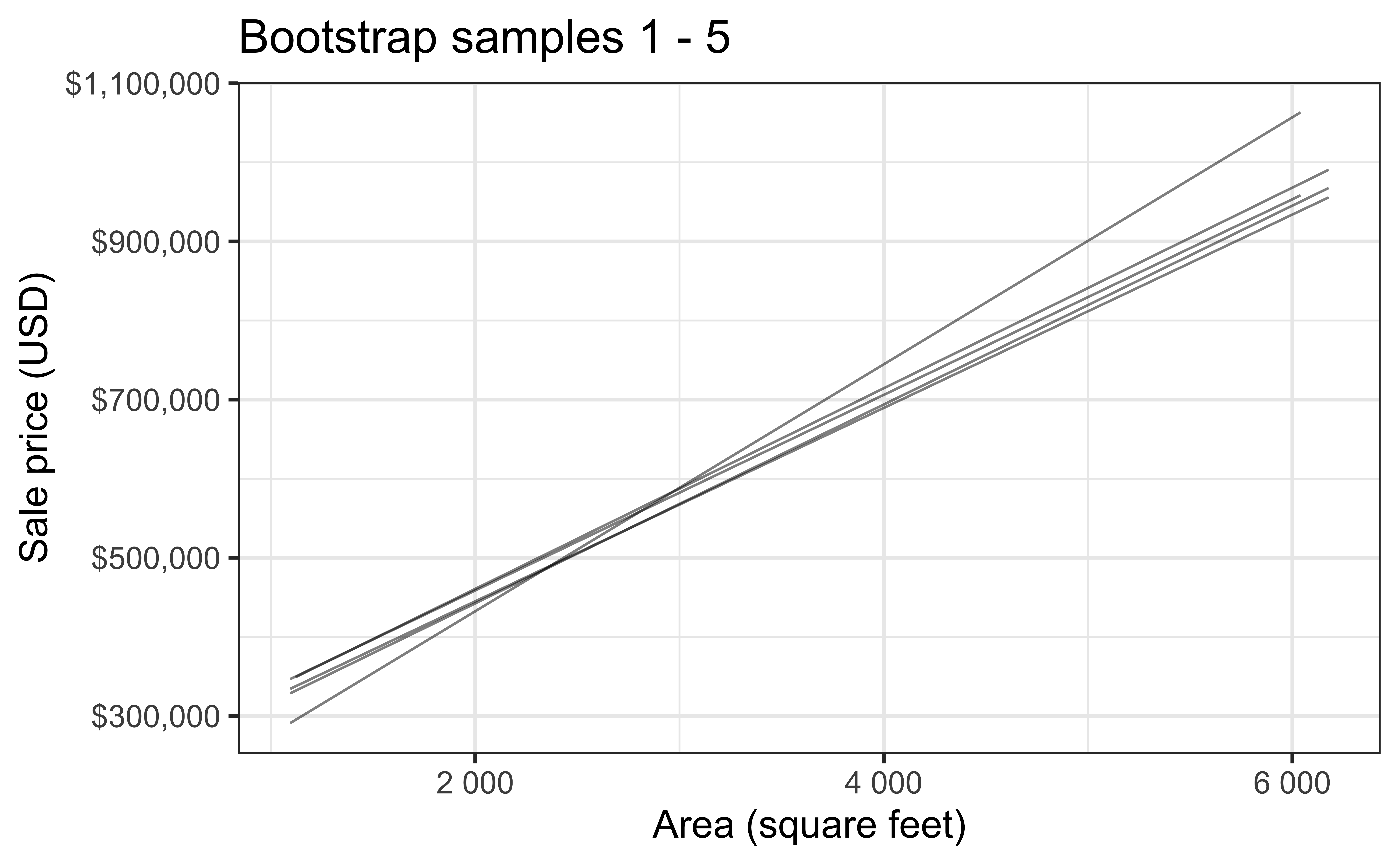
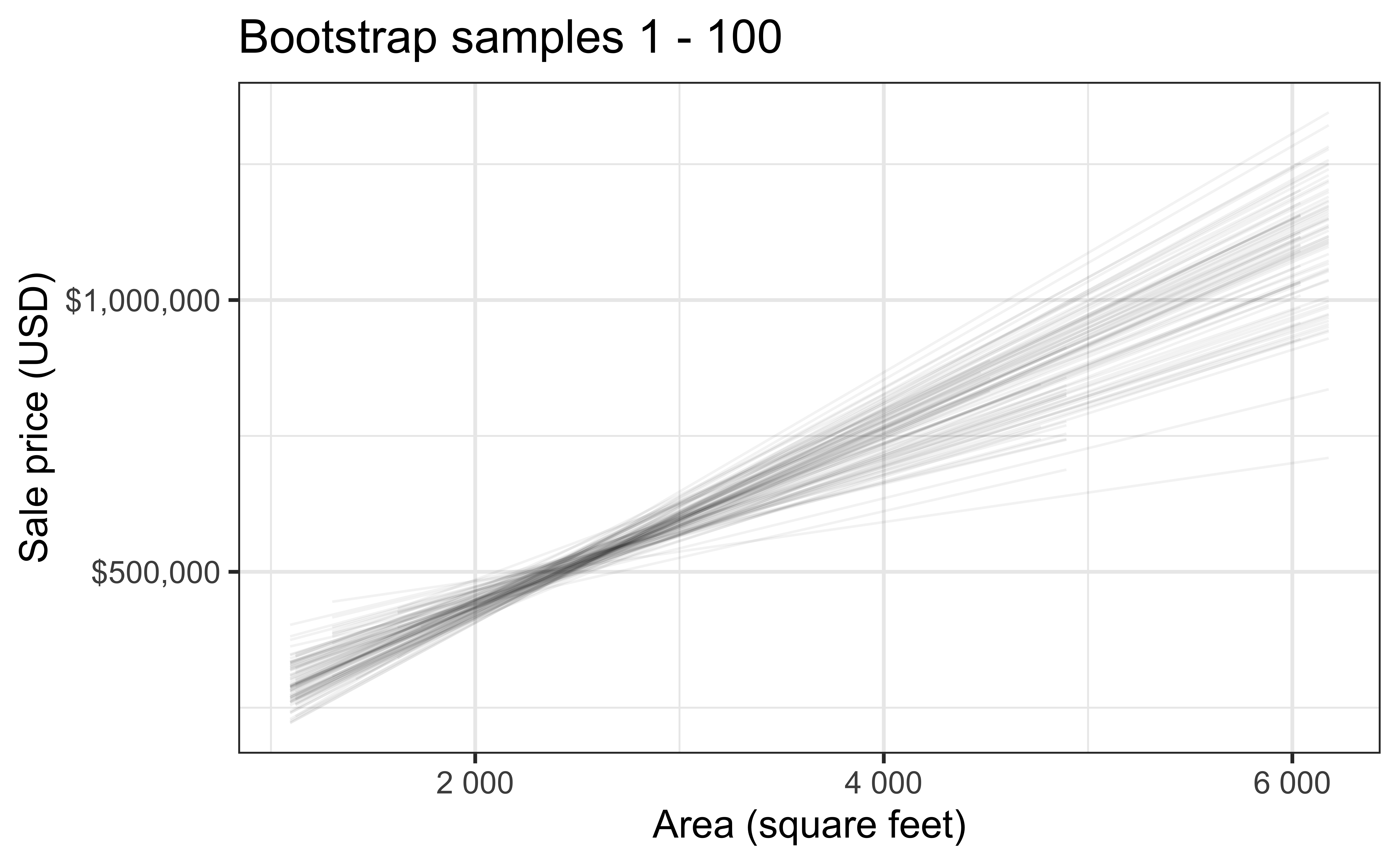
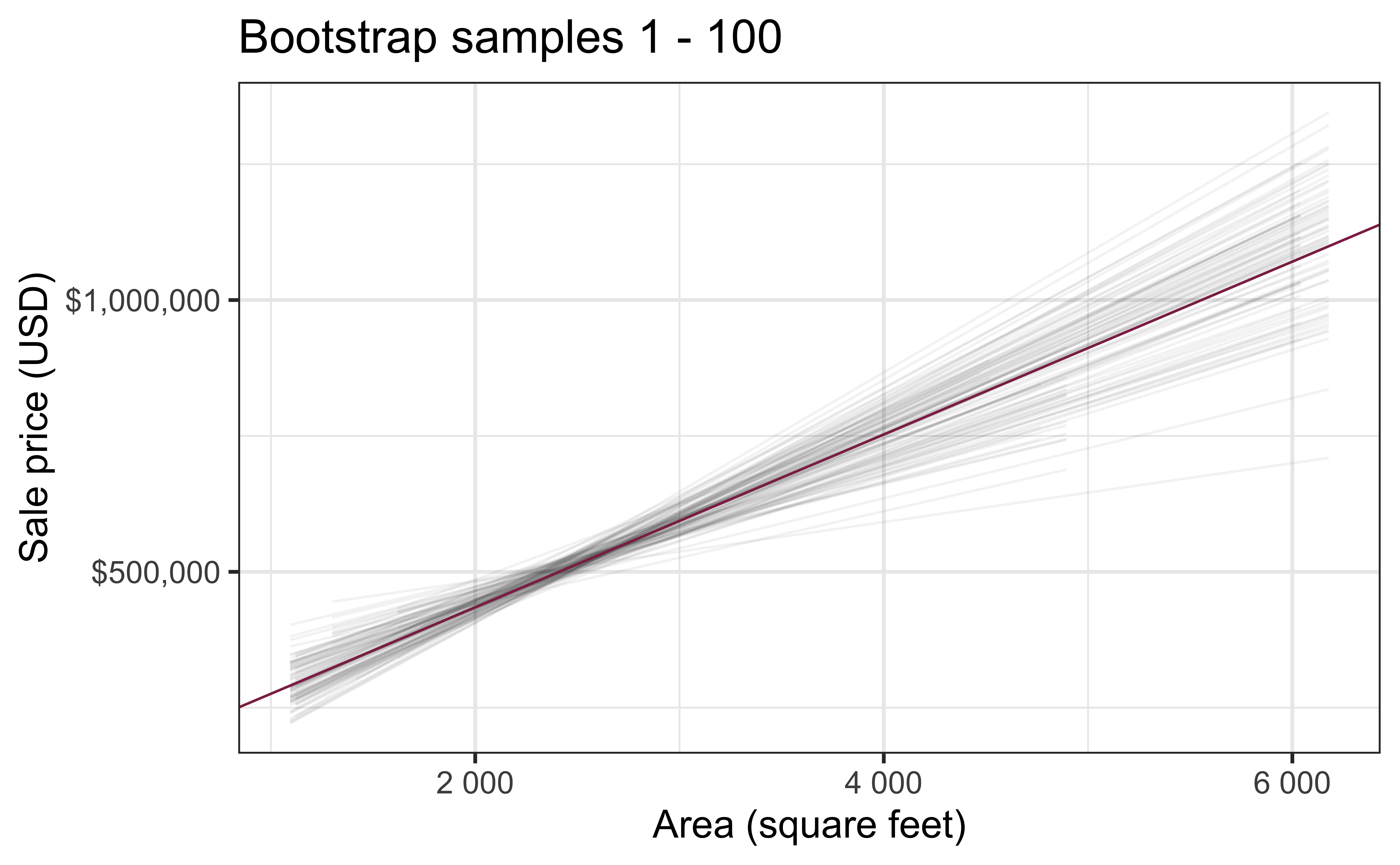
Bootstrap samples 1 - 5

Bootstrap samples 1 - 100

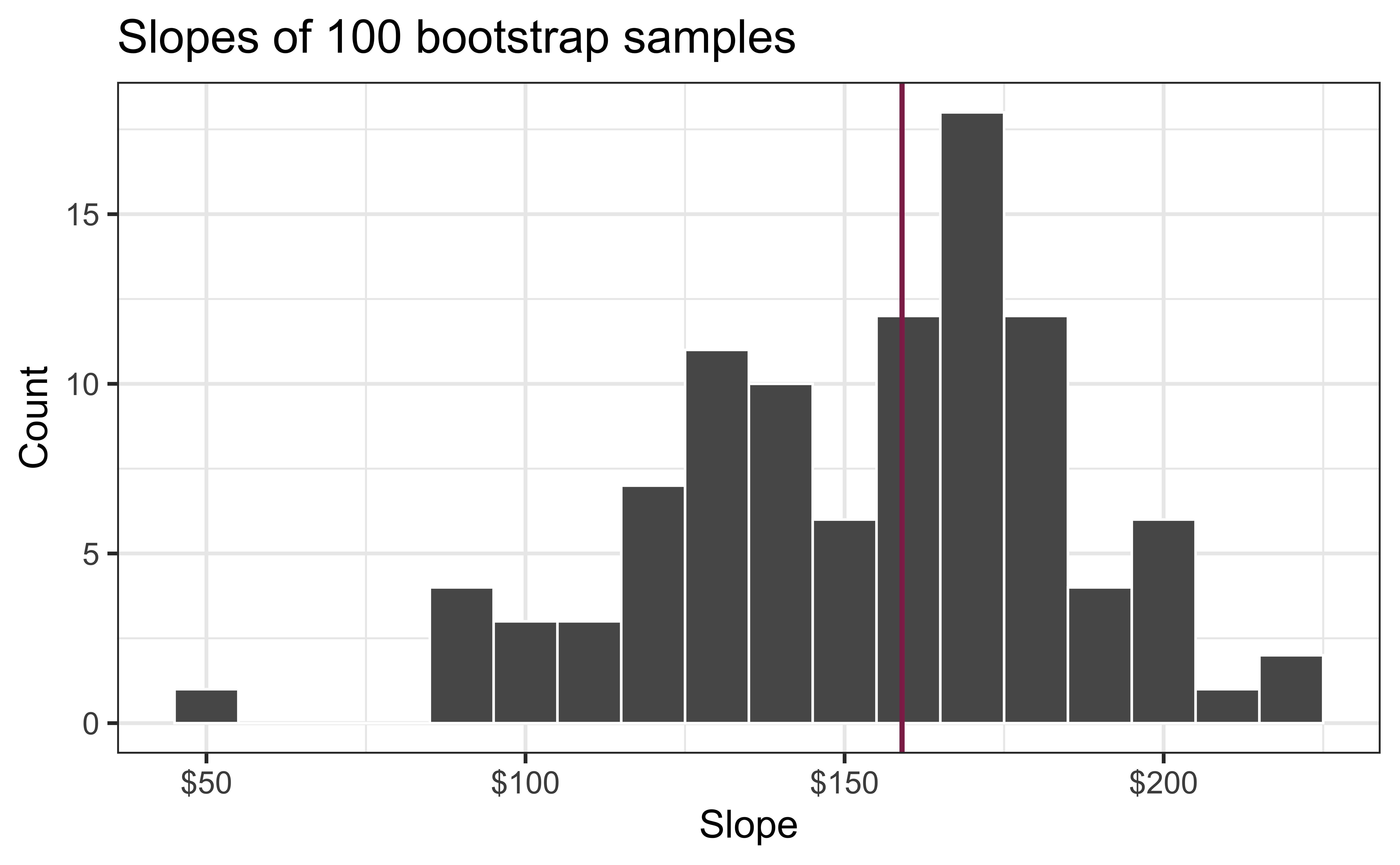
Slopes of bootstrap samples

Fill in the blank: For each additional square foot, the model predicts the sale price of Duke Forest houses to be higher, on average, by $159, plus or minus ___ dollars.

Slopes of bootstrap samples

Fill in the blank: For each additional square foot, the model predicts the sale price of Duke Forest houses to be higher, on average, by $159, plus or minus ___ dollars.

Confidence level

How confident are you that the true slope is between $0 and $250? How about $150 and $170? How about $90 and $210?

95% confidence interval

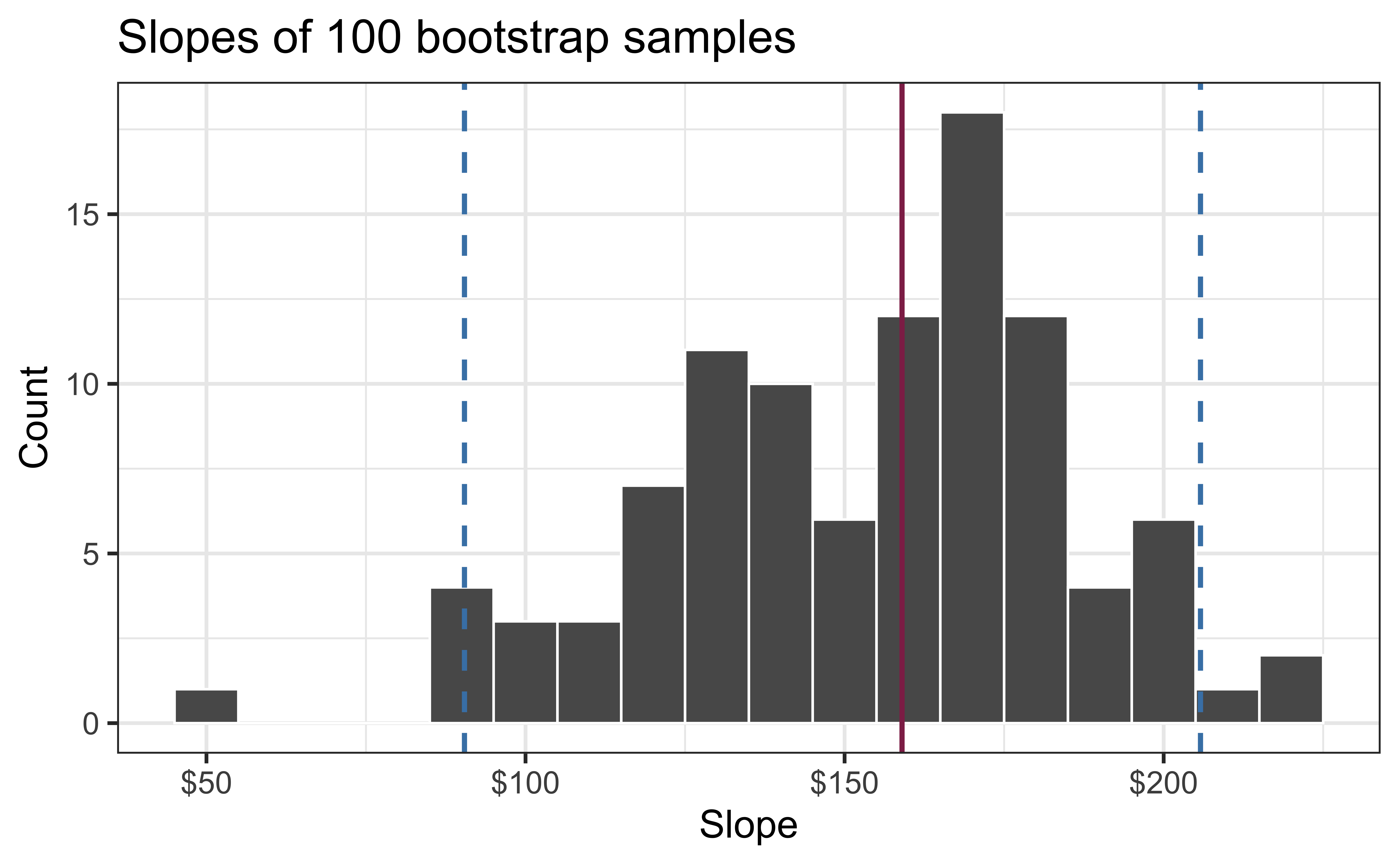
• A 95% confidence interval is bounded by the middle 95% of the bootstrap distribution
• We are 95% confident that for each additional square foot, the model predicts the sale price of Duke Forest houses to be higher, on average, by $90.43 to $205.77.

Application exercise

📋 AE 03: Bootstrap confidence intervals

Computing the CI for the slope I

Calculate the observed slope:

observed_fit <- duke_forest |>
  specify(price ~ area) |>
  fit()

observed_fit

# A tibble: 2 × 2
  term      estimate
  <chr>        <dbl>
1 intercept  116652.
2 area          159.

Computing the CI for the slope II

Take 100 bootstrap samples and fit models to each one:

set.seed(1120)

boot_fits <- duke_forest |>
  specify(price ~ area) |>
  generate(reps = 100, type = "bootstrap") |>
  fit()

boot_fits

# A tibble: 200 × 3
# Groups:   replicate [100]
   replicate term      estimate
       <int> <chr>        <dbl>
 1         1 intercept   47819.
 2         1 area          191.
 3         2 intercept  144645.
 4         2 area          134.
 5         3 intercept  114008.
 6         3 area          161.
 7         4 intercept  100639.
 8         4 area          166.
 9         5 intercept  215264.
10         5 area          125.
# … with 190 more rows

Computing the CI for the slope III

Percentile method: Compute the 95% CI as the middle 95% of the bootstrap distribution:

get_confidence_interval(
  boot_fits, 
  point_estimate = observed_fit, 
  level = 0.95,
  type = "percentile"
)

# A tibble: 2 × 3
  term      lower_ci upper_ci
  <chr>        <dbl>    <dbl>
1 area          92.1     223.
2 intercept -36765.   296528.

Computing the CI for the slope IV

Standard error method: Alternatively, compute the 95% CI as the point estimate \(\pm\) ~2 standard deviations of the bootstrap distribution:

get_confidence_interval(
  boot_fits, 
  point_estimate = observed_fit, 
  level = 0.95,
  type = "se"
)

# A tibble: 2 × 3
  term      lower_ci upper_ci
  <chr>        <dbl>    <dbl>
1 area          90.8     228.
2 intercept -56788.   290093.

Precision vs. accuracy

If we want to be very certain that we capture the population parameter, should we use a wider or a narrower interval? What drawbacks are associated with using a wider interval?

Precision vs. accuracy

How can we get best of both worlds – high precision and high accuracy?

Changing confidence level

How would you modify the following code to calculate a 90% confidence interval? How would you modify it for a 99% confidence interval?

get_confidence_interval(
  boot_fits, 
  point_estimate = observed_fit, 
  level = 0.95,
  type = "percentile"
)

# A tibble: 2 × 3
  term      lower_ci upper_ci
  <chr>        <dbl>    <dbl>
1 area          92.1     223.
2 intercept -36765.   296528.

Changing confidence level

## confidence level: 90%
get_confidence_interval(
  boot_fits, point_estimate = observed_fit, 
  level = 0.90, type = "percentile"
)

# A tibble: 2 × 3
  term      lower_ci upper_ci
  <chr>        <dbl>    <dbl>
1 area          104.     212.
2 intercept  -24380.  256730.

## confidence level: 99%
get_confidence_interval(
  boot_fits, point_estimate = observed_fit, 
  level = 0.99, type = "percentile"
)

# A tibble: 2 × 3
  term      lower_ci upper_ci
  <chr>        <dbl>    <dbl>
1 area          56.3     226.
2 intercept -61950.   370395.

Recap

• Population: Complete set of observations of whatever we are studying, e.g., people, tweets, photographs, etc. (population size = \(N\))

• Sample: Subset of the population, ideally random and representative (sample size = \(n\))

• Sample statistic \(\ne\) population parameter, but if the sample is good, it can be a good estimate

• Statistical inference: Discipline that concerns itself with the development of procedures, methods, and theorems that allow us to extract meaning and information from data that has been generated by stochastic (random) process

• We report the estimate with a confidence interval, and the width of this interval depends on the variability of sample statistics from different samples from the population

• Since we can’t continue sampling from the population, we bootstrap from the one sample we have to estimate sampling variability