library(tidyverse)
library(tidymodels)
library(openintro)
library(knitr)AE 03: Bootstrap confidence intervals
Houses in Duke Forest
Important
Go to the course GitHub organization and locate your ae-03-bootstrap- to get started.
The AE is due on GitHub by Thursday, September 15 at 11:59pm.
Data
The data are on houses that were sold in the Duke Forest neighborhood of Durham, NC around November 2020. It was originally scraped from Zillow, and can be found in the duke_forest data set in the openintro R package.
glimpse(duke_forest)Rows: 98
Columns: 13
$ address <chr> "1 Learned Pl, Durham, NC 27705", "1616 Pinecrest Rd, Durha…
$ price <dbl> 1520000, 1030000, 420000, 680000, 428500, 456000, 1270000, …
$ bed <dbl> 3, 5, 2, 4, 4, 3, 5, 4, 4, 3, 4, 4, 3, 5, 4, 5, 3, 4, 4, 3,…
$ bath <dbl> 4.0, 4.0, 3.0, 3.0, 3.0, 3.0, 5.0, 3.0, 5.0, 2.0, 3.0, 3.0,…
$ area <dbl> 6040, 4475, 1745, 2091, 1772, 1950, 3909, 2841, 3924, 2173,…
$ type <chr> "Single Family", "Single Family", "Single Family", "Single …
$ year_built <dbl> 1972, 1969, 1959, 1961, 2020, 2014, 1968, 1973, 1972, 1964,…
$ heating <chr> "Other, Gas", "Forced air, Gas", "Forced air, Gas", "Heat p…
$ cooling <fct> central, central, central, central, central, central, centr…
$ parking <chr> "0 spaces", "Carport, Covered", "Garage - Attached, Covered…
$ lot <dbl> 0.97, 1.38, 0.51, 0.84, 0.16, 0.45, 0.94, 0.79, 0.53, 0.73,…
$ hoa <chr> NA, NA, NA, NA, NA, NA, NA, NA, NA, NA, NA, NA, NA, NA, NA,…
$ url <chr> "https://www.zillow.com/homedetails/1-Learned-Pl-Durham-NC-…Exploratory data analysis
ggplot(duke_forest, aes(x = area, y = price)) +
  geom_point(alpha = 0.7) +
  labs(
    x = "Area (square feet)",
    y = "Sale price (USD)",
    title = "Price and area of houses in Duke Forest"
  ) +
scale_y_continuous(labels = label_dollar()) 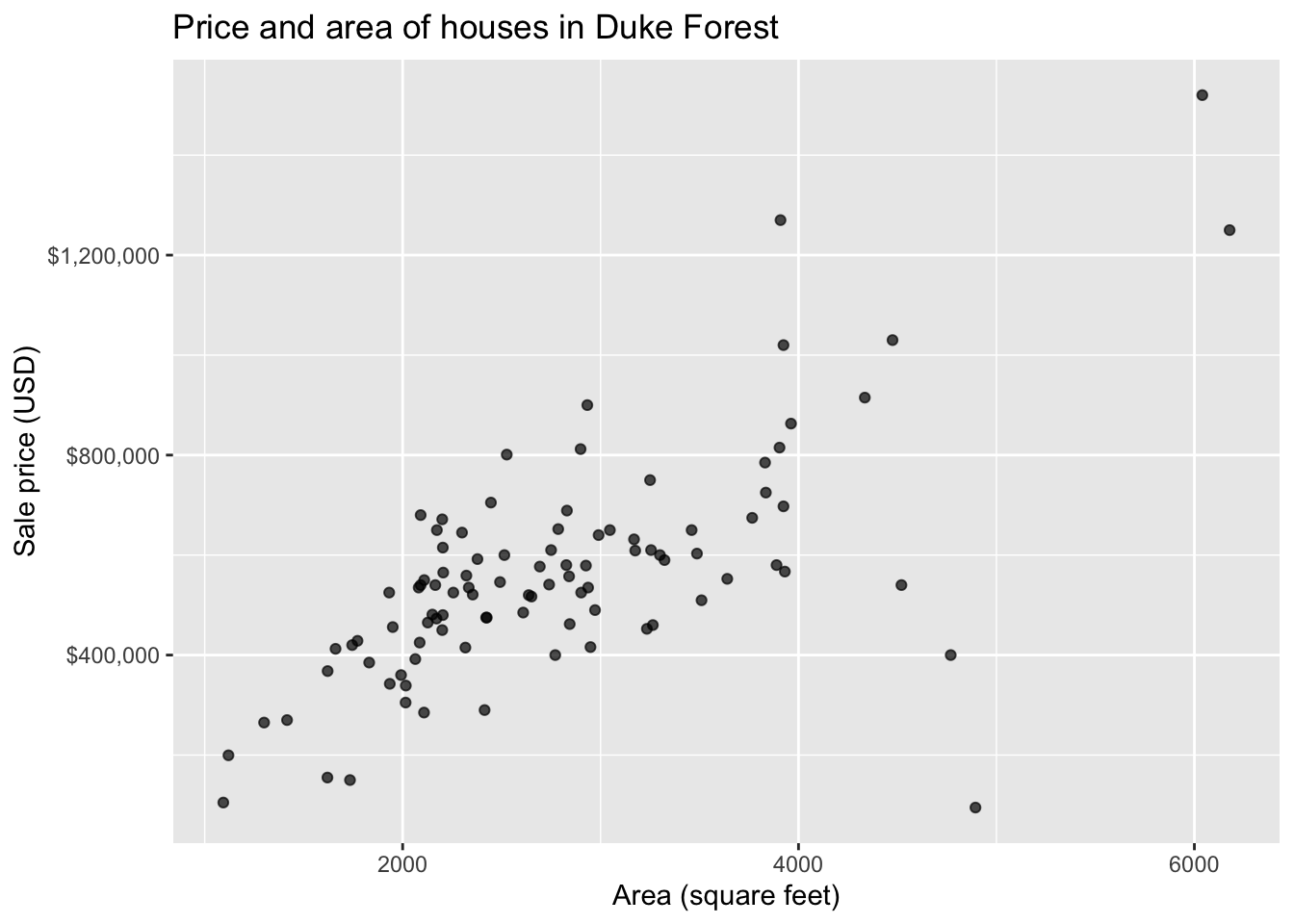
Model
df_fit <- linear_reg() |>
  set_engine("lm") |>
  fit(price ~ area, data = duke_forest)

tidy(df_fit) |>
kable(digits = 2)| term | estimate | std.error | statistic | p.value |
|---|---|---|---|---|
| (Intercept) | 116652.33 | 53302.46 | 2.19 | 0.03 |
| area | 159.48 | 18.17 | 8.78 | 0.00 |
Bootstrap confidence interval
1. Calculate the observed fit (slope)
observed_fit <- duke_forest |>
  specify(price ~ area) |>
  fit()

observed_fit
# A tibble: 2 × 2
term estimate
<chr> <dbl>
1 intercept 116652.
2 area 159.2 Take n bootstrap samples and fit models to each one.
Fill in the code, then set eval: true .
n = 100
set.seed(091222)

boot_fits <- ______ |>
  specify(______) |>
  generate(reps = ____, type = "bootstrap") |>
  fit()

boot_fits
Why do we set a seed before taking the bootstrap samples?
Make a histogram of the bootstrap samples to visualize the bootstrap distribution.
# Code for histogram
3 Compute the 95% confidence interval as the middle 95% of the bootstrap distribution
Fill in the code, then set eval: true .
get_confidence_interval(
  boot_fits,
  point_estimate = _____,
  level = ____,
  type = "percentile"
)
Changing confidence level
Modify the code from Step 3 to create a 90% confidence interval.
# Paste code for 90% confidence intervalModify the code from Step 3 to create a 99% confidence interval.
# Paste code for 90% confidence intervalWhich confidence level produces the most accurate confidence interval (90%, 95%, 99%)? Explain
Which confidence level produces the most precise confidence interval (90%, 95%, 99%)? Explain
If we want to be very certain that we capture the population parameter, should we use a wider or a narrower interval? What drawbacks are associated with using a wider interval?
If we want to be very certain that we capture the population parameter, should we use a wider or a narrower interval? What drawbacks are associated with using a wider interval?
Important
To submit the AE:
- Render the document to produce the PDF with all of your work from today’s class.
- Push all your work to your
ae-03-repo on GitHub. (You do not submit AEs on Gradescope).