MLR conditions + multicollinearity

Prof. Maria Tackett

Oct 31, 2022

Announcements

Project proposal due Fri, Nov 04
HW 03 due Mon, Nov 07 at 11:59pm
- Released later today
See Week 10 activities

Topics

Conditions for inference
Multicollinearity

Computational setup

# load packages
library(tidyverse)
library(tidymodels)
library(knitr)      # for tables
library(patchwork)  # for laying out plots
library(rms)        # for vif

# set default theme and larger font size for ggplot2
ggplot2::theme_set(ggplot2::theme_bw(base_size = 20))

Data: `rail_trail`

The Pioneer Valley Planning Commission (PVPC) collected data for ninety days from April 5, 2005 to November 15, 2005.
Data collectors set up a laser sensor, with breaks in the laser beam recording when a rail-trail user passed the data collection station.

rail_trail <- read_csv(here::here("slides", "data/rail_trail.csv"))
rail_trail

# A tibble: 90 × 7
   volume hightemp avgtemp season cloudcover precip day_type
    <dbl>    <dbl>   <dbl> <chr>       <dbl>  <dbl> <chr>   
 1    501       83    66.5 Summer       7.60 0      Weekday 
 2    419       73    61   Summer       6.30 0.290  Weekday 
 3    397       74    63   Spring       7.5  0.320  Weekday 
 4    385       95    78   Summer       2.60 0      Weekend 
 5    200       44    48   Spring      10    0.140  Weekday 
 6    375       69    61.5 Spring       6.60 0.0200 Weekday 
 7    417       66    52.5 Spring       2.40 0      Weekday 
 8    629       66    52   Spring       0    0      Weekend 
 9    533       80    67.5 Summer       3.80 0      Weekend 
10    547       79    62   Summer       4.10 0      Weekday 
# … with 80 more rows

Source: Pioneer Valley Planning Commission via the mosaicData package.

Variables

Outcome:

volume estimated number of trail users that day (number of breaks recorded)

Predictors

hightemp daily high temperature (in degrees Fahrenheit)
avgtemp average of daily low and daily high temperature (in degrees Fahrenheit)
season one of “Fall”, “Spring”, or “Summer”
cloudcover measure of cloud cover (in oktas)
precip measure of precipitation (in inches)
day_type one of “weekday” or “weekend”

Conditions for inference

Full model

Including all available predictors

Fit:

rt_full_fit <- linear_reg() |>
  set_engine("lm") |>
  fit(volume ~ ., data = rail_trail)

Summarize:

tidy(rt_full_fit)

# A tibble: 8 × 5
  term            estimate std.error statistic p.value
  <chr>              <dbl>     <dbl>     <dbl>   <dbl>
1 (Intercept)        17.6      76.6      0.230 0.819  
2 hightemp            7.07      2.42     2.92  0.00450
3 avgtemp            -2.04      3.14    -0.648 0.519  
4 seasonSpring       35.9      33.0      1.09  0.280  
5 seasonSummer       24.2      52.8      0.457 0.649  
6 cloudcover         -7.25      3.84    -1.89  0.0627 
7 precip            -95.7      42.6     -2.25  0.0273 
8 day_typeWeekend    35.9      22.4      1.60  0.113

Augment:

rt_full_aug <- augment(rt_full_fit$fit)

Model conditions

Linearity: There is a linear relationship between the response and predictor variables.
Constant Variance: The variability about the least squares line is generally constant.
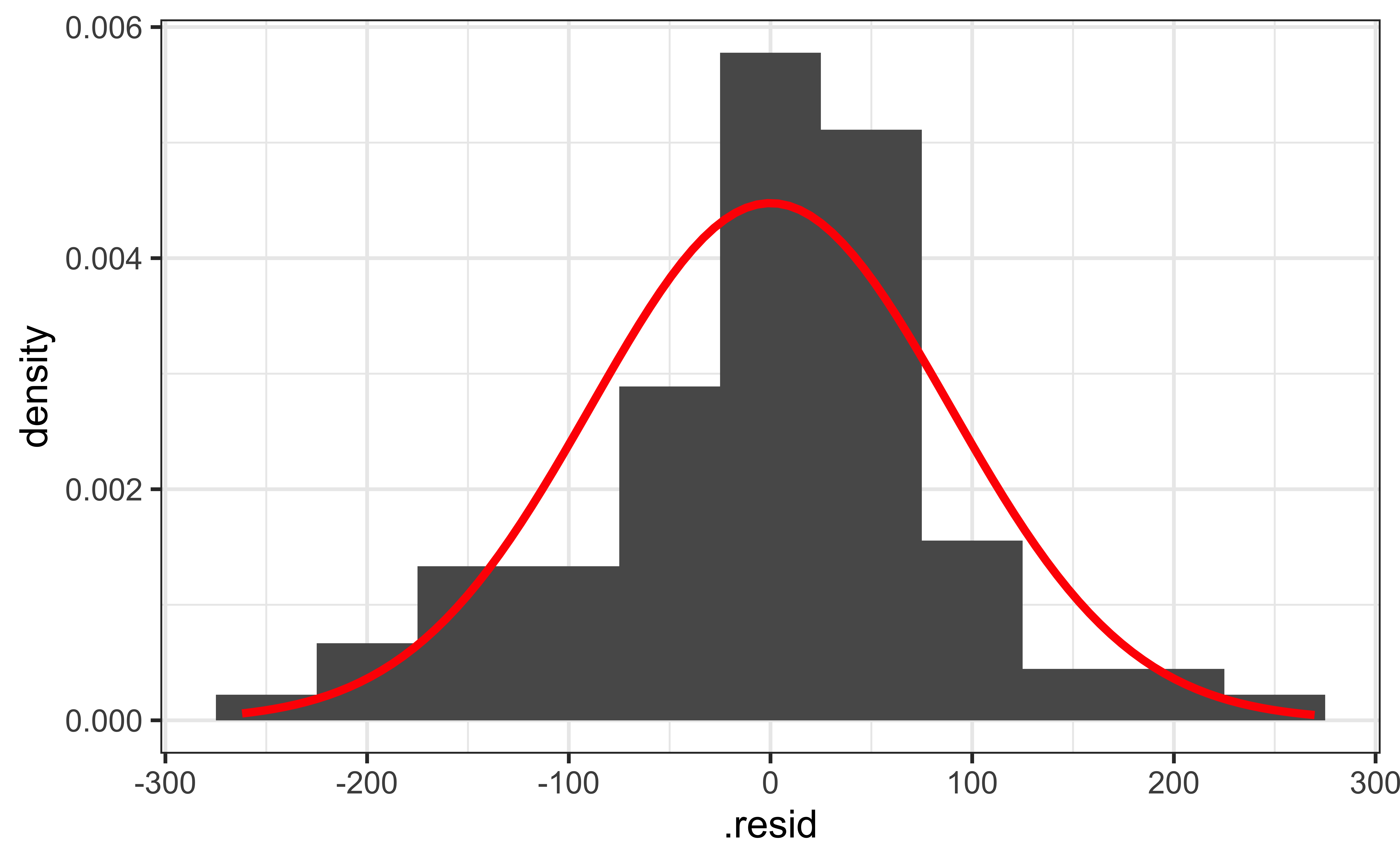
Normality: The distribution of the residuals is approximately normal.
Independence: The residuals are independent from each other.

Residuals vs. predicted values

ggplot(data = rt_full_aug, aes(x = .fitted, y = .resid)) +
  geom_point(alpha = 0.7) +
  geom_hline(yintercept = 0, color = "red", linetype = "dashed") +
  labs(x = "Predicted values", y = "Residuals")

Linearity: Residuals vs. predicted

Does the linearity condition appear to be met?

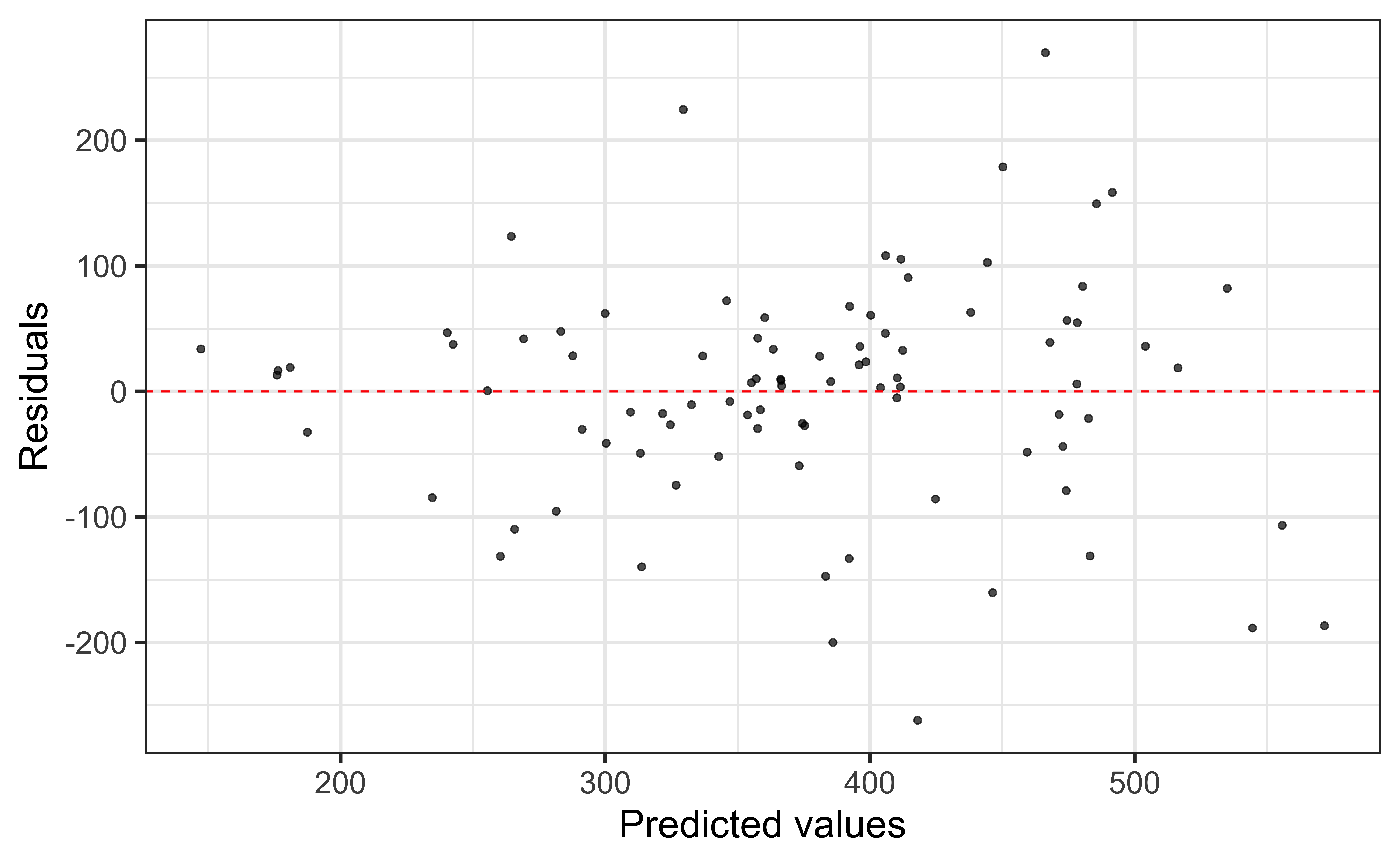
Linearity: Residuals vs. predicted

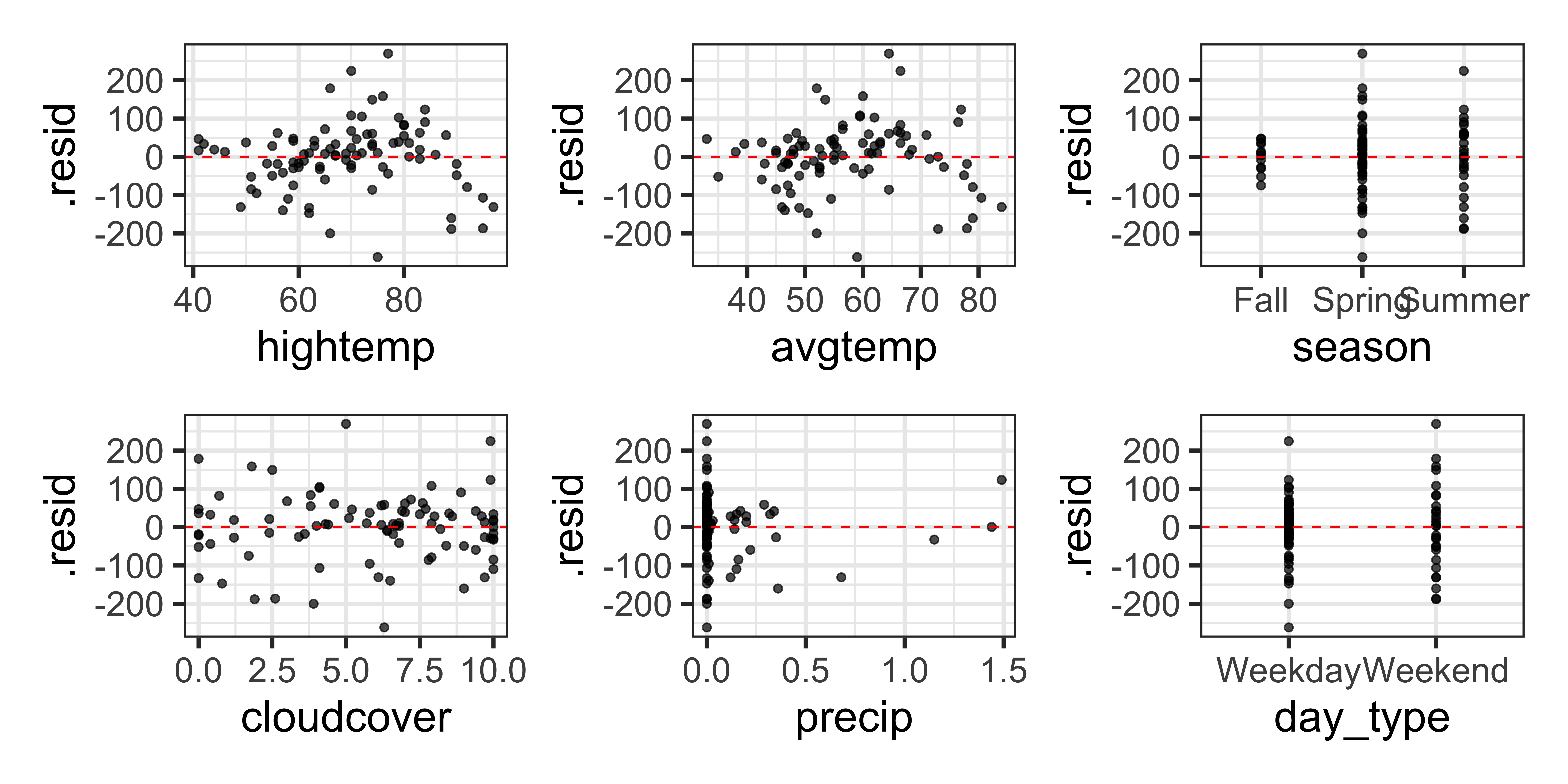
Look at individual plots of residuals vs. each predictor, particularly if there are potential issues in the plot of residuals vs. predicted values.

Linearity: Residuals vs. each predictor

Checking linearity

The plots of residuals vs. hightemp and avgtemp appear to have a parabolic pattern.
The linearity condition is not satisfied given these plots.

Checking constant variance

Does the constant variance condition appear to be satisfied?

Checking constant variance

The vertical spread of the residuals is not constant across the plot.
The constant variance condition is not satisfied.

Checking normality

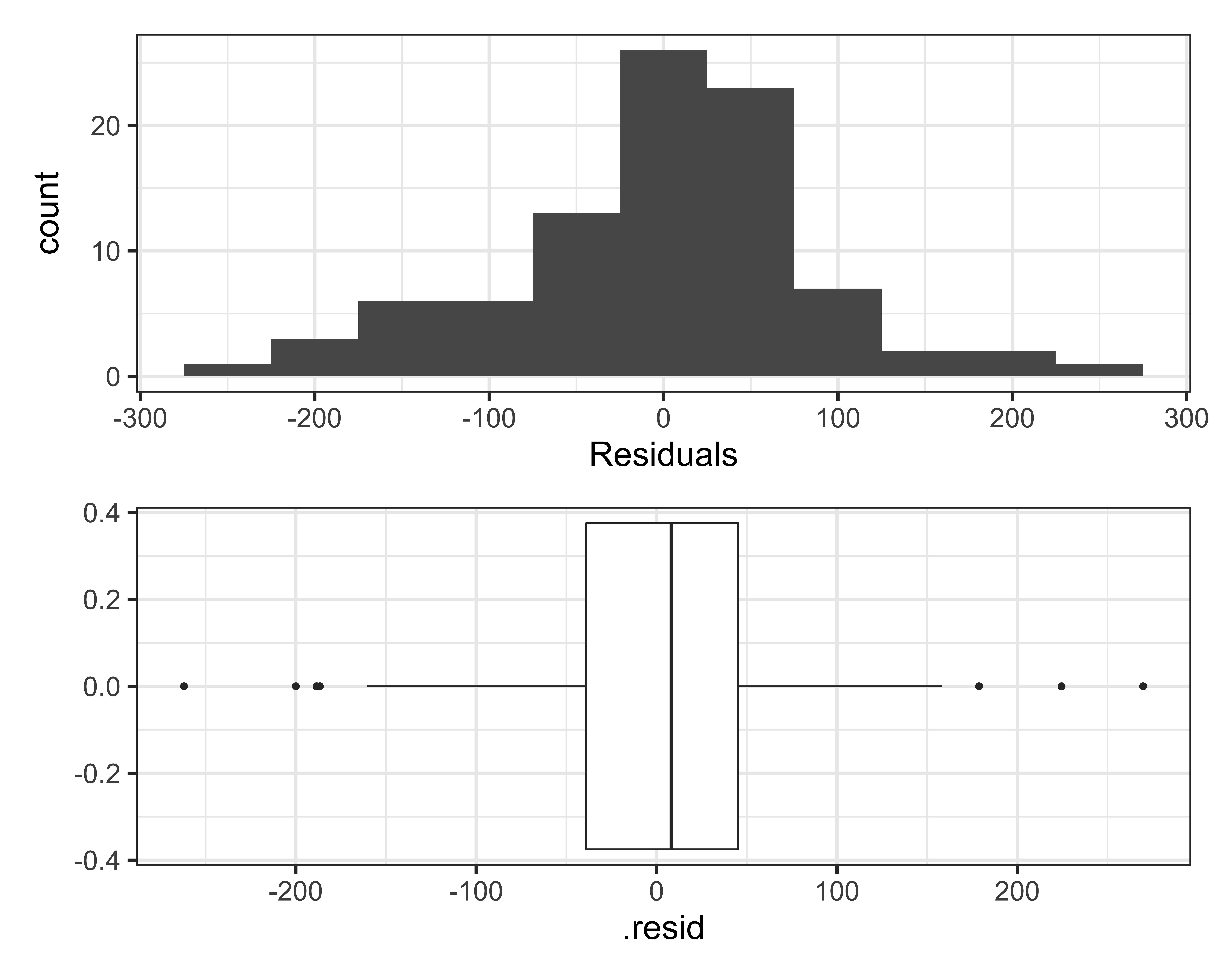
Overlaying a density plot on a histogram

📋 AE 11: MLR Inference

Ex 2. Fill in the code to recreate the following visualization in R based on the results of the model.

Checking independence

We can often check the independence condition based on the context of the data and how the observations were collected.
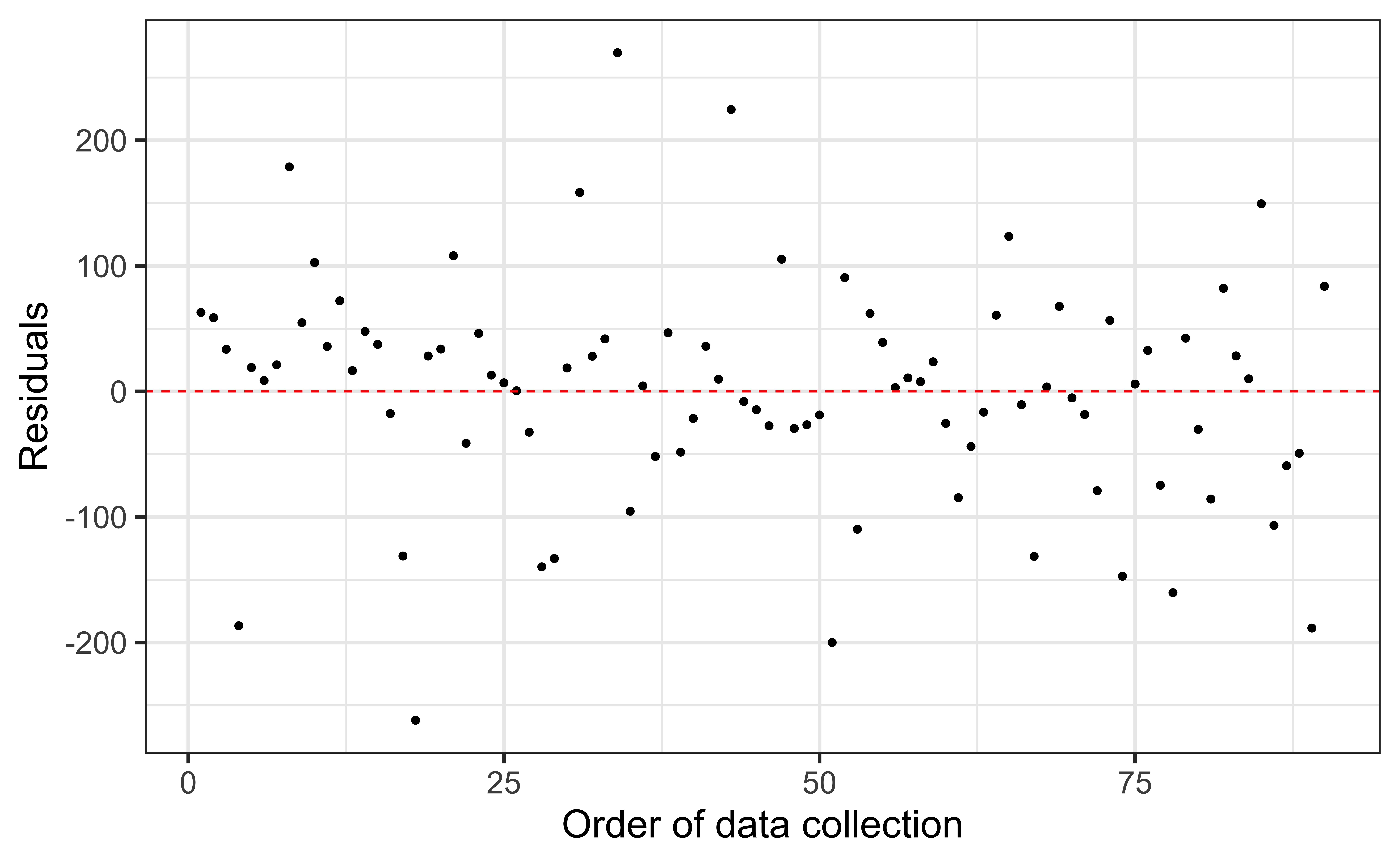
If the data were collected in a particular order, examine a scatterplot of the residuals versus order in which the data were collected.
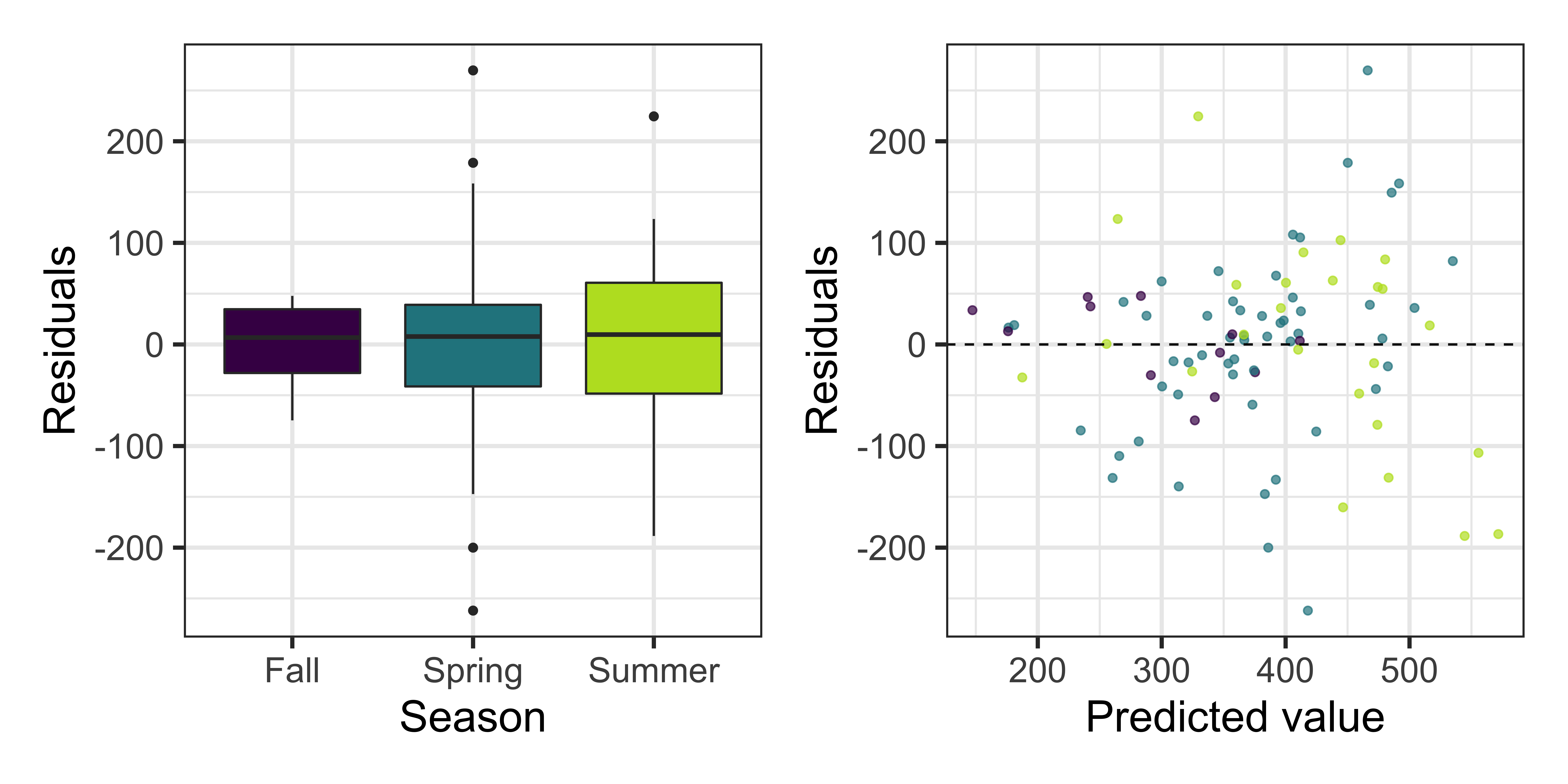
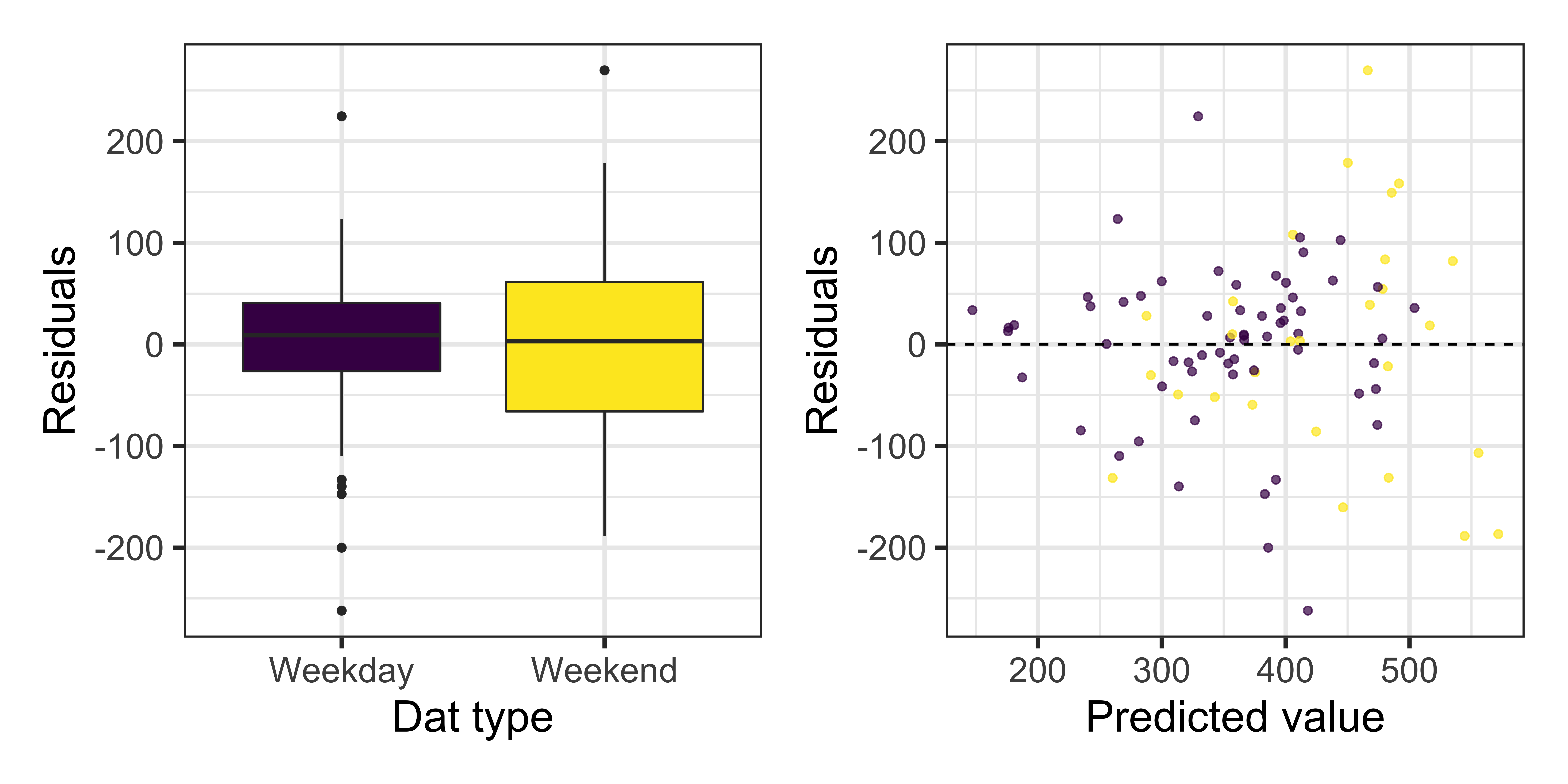
If there is a grouping variable lurking in the background, check the residuals based on that grouping variable.

Checking independence

Residuals vs. order of data collection:

ggplot(rt_full_aug, aes(y = .resid, x = 1:nrow(rt_full_aug))) +
  geom_point() +
  geom_hline(yintercept = 0, color = "red", linetype = "dashed") +
  labs(x = "Order of data collection", y = "Residuals")

Checking independence

Residuals vs. predicted values by season:

Checking independence

Residuals vs. predicted values by day_type:

Checking independence

No clear pattern in the residuals vs. order of data collection plot and the model predicts similarly for seasons and day types.
Independence condition appears to be satisfied, as far as we can evaluate it.

Multicollinearity

Why multicollinearity is a problem

We can’t include two variables that have a perfect linear association with each other
If we did so, we could not find unique estimates for the model coefficients

Example

Suppose the true population regression equation is \(y = 3 + 4x\)

Suppose we try estimating that equation using a model with variables \(x\) and \(z = x/10\)

\[ \begin{aligned}\hat{y}&= \hat{\beta}_0 + \hat{\beta}_1x + \hat{\beta}_2z\\ &= \hat{\beta}_0 + \hat{\beta}_1x + \hat{\beta}_2\frac{x}{10}\\ &= \hat{\beta}_0 + \bigg(\hat{\beta}_1 + \frac{\hat{\beta}_2}{10}\bigg)x \end{aligned} \]

Example

\[\hat{y} = \hat{\beta}_0 + \bigg(\hat{\beta}_1 + \frac{\hat{\beta}_2}{10}\bigg)x\]

We can set \(\hat{\beta}_1\) and \(\hat{\beta}_2\) to any two numbers such that \(\hat{\beta}_1 + \frac{\hat{\beta}_2}{10} = 4\)
Therefore, we are unable to choose the “best” combination of \(\hat{\beta}_1\) and \(\hat{\beta}_2\)

Why multicollinearity is a problem

When we have almost perfect collinearities (i.e. highly correlated predictor variables), the standard errors for our regression coefficients inflate
In other words, we lose precision in our estimates of the regression coefficients
This impedes our ability to use the model for inference or prediction

Detecting Multicollinearity

Multicollinearity may occur when…

There are very high correlations \((r > 0.9)\) among two or more predictor variables, especially when the sample size is small

One (or more) predictor variables is an almost perfect linear combination of the others
Include a quadratic in the model mean-centering the variable first
Including interactions between two or more continuous variables

Detecting multicollinearity in the EDA

Look at a correlation matrix of the predictor variables, including all indicator variables
- Look out for values close to 1 or -1
Look at a scatterplot matrix of the predictor variables
- Look out for plots that show a relatively linear relationship

Detecting Multicollinearity (VIF)

Variance Inflation Factor (VIF): Measure of multicollinearity in the regression model

\[VIF(\hat{\beta}_j) = \frac{1}{1-R^2_{X_j|X_{-j}}}\]

where \(R^2_{X_j|X_{-j}}\) is the proportion of variation \(X\) that is explained by the linear combination of the other explanatory variables in the model.

Detecting Multicollinearity (VIF)

Typically \(VIF > 10\) indicates concerning multicollinearity - Variables with similar values of VIF are typically the ones correlated with each other

Use the vif() function in the rms R package to calculate VIF

VIF for rail trail model

vif(rt_full_fit$fit)

       hightemp         avgtemp    seasonSpring    seasonSummer      cloudcover 
      10.259978       13.086175        2.751577        5.841985        1.587485 
         precip day_typeWeekend 
       1.295352        1.125741

hightemp and avgtemp are correlated. We need to remove one of these variables and refit the model.

Model without `hightemp`

m1 <- linear_reg() |>
  set_engine("lm") |>
  fit(volume ~ . - hightemp, data = rail_trail)
  
m1 |>
  tidy() |>
  kable(digits = 3)

term	estimate	std.error	statistic	p.value
(Intercept)	76.071	77.204	0.985	0.327
avgtemp	6.003	1.583	3.792	0.000
seasonSpring	34.555	34.454	1.003	0.319
seasonSummer	13.531	55.024	0.246	0.806
cloudcover	-12.807	3.488	-3.672	0.000
precip	-110.736	44.137	-2.509	0.014
day_typeWeekend	48.420	22.993	2.106	0.038

Model without `avgtemp`

m2 <- linear_reg() |>
  set_engine("lm") |>
  fit(volume ~ . - avgtemp, data = rail_trail)
  
m2 |>
  tidy() |>
  kable(digits = 3)

term	estimate	std.error	statistic	p.value
(Intercept)	8.421	74.992	0.112	0.911
hightemp	5.696	1.164	4.895	0.000
seasonSpring	31.239	32.082	0.974	0.333
seasonSummer	9.424	47.504	0.198	0.843
cloudcover	-8.353	3.435	-2.431	0.017
precip	-98.904	42.137	-2.347	0.021
day_typeWeekend	37.062	22.280	1.663	0.100

Choosing a model

Model with hightemp removed:

adj.r.squared	AIC	BIC
0.42	1087.5	1107.5

Model with avgtemp removed:

adj.r.squared	AIC	BIC
0.47	1079.05	1099.05

Based on Adjusted \(R^2\), AIC, and BIC, the model with avgtemp removed is a better fit. Therefore, we choose to remove avgtemp from the model and leave hightemp in the model to deal with the multicollinearity.

Final model

term	estimate	std.error	statistic	p.value
(Intercept)	8.421	74.992	0.112	0.911
hightemp	5.696	1.164	4.895	0.000
seasonSpring	31.239	32.082	0.974	0.333
seasonSummer	9.424	47.504	0.198	0.843
cloudcover	-8.353	3.435	-2.431	0.017
precip	-98.904	42.137	-2.347	0.021
day_typeWeekend	37.062	22.280	1.663	0.100

Recap

Conditions for inference
Multicollinearity

Application exercise

📋 AE 12: Multiple Linear Regression Review

MLR conditions + multicollinearity

Announcements

Topics

Computational setup

Data: rail_trail

Variables

Conditions for inference

Full model

Model conditions

Residuals vs. predicted values

Linearity: Residuals vs. predicted

Linearity: Residuals vs. predicted

Linearity: Residuals vs. each predictor

Checking linearity

Checking constant variance

Checking constant variance

Checking normality

Overlaying a density plot on a histogram

Checking independence

Checking independence

Checking independence

Checking independence

Checking independence

Multicollinearity

Why multicollinearity is a problem

Example

Example

Why multicollinearity is a problem

Detecting Multicollinearity

Detecting multicollinearity in the EDA

Detecting Multicollinearity (VIF)

Detecting Multicollinearity (VIF)

VIF for rail trail model

Model without hightemp

Model without avgtemp

Choosing a model

Final model

Recap

Application exercise

Data: `rail_trail`

Model without `hightemp`

Model without `avgtemp`