03:00
Introduction to multilevel models
Prof. Maria Tackett
Nov 28, 2022
Announcements
Due dates
- Statistics experience due Fri, Dec 09, 11:59pm
Exam 02: Mon, Dec 05 (evening) - Thu, Dec 08, 12pm (noon)
Exam 02 review on Mon Dec 05
Click here for lecture recordings - available until Dec 05, 11:59pm
See Week 14 activities
Learning goals
- Recognize a potential for correlation in a data set
- Identify observational units at varying levels
- Understand issues correlated data may cause in modeling
- Understand how random effects models can be used to take correlation into account
Correlated observations
Examples of correlated data
- In an education study, scores for students from a particular teacher are typically more similar than scores of other students with a different teacher
- In a study measuring depression indices weekly over a month, the four measures for the same patient tend to be more similar than depression indices from other patients
- In political polling, opinions of members from the same household tend to be more similar than opinions of members from another household
Correlation among outcomes within the same group (teacher, patient, household) is called intraclass correlation
Multilevel data
We can think of correlated data as having a multilevel structure
- Population elements are aggregated into groups
- There are observational units and measurements at each level
For now we will focus on data with two levels:
- Level one: Most basic level of observation
- Level two: Groups formed from aggregated level-one observations
- Example: education
- Level one: students in a class
- Level two: class / teacher
Two types of effects
- Fixed effects: Effects that are of interest in the study
- Can think of these as effects whose interpretations would be included in a write up of the study
- Random effects: Effects we’re not interested in studying but whose variability we want to understand
- Can think of these as effects whose interpretations would not necessarily be included in a write up of the study
Example
Researchers are interested in understanding the effect social media has on opinions about a proposed economic plan. They randomly select 1000 households. They ask each adult in the household how many minutes they spend on social media daily and whether they support the proposed economic plan.
- Fixed effect: daily minutes on social media
- Random effect: household
Practice
Researchers conducted a randomized controlled study where patients were randomly assigned to either an anti-epileptic drug or a placebo. For each patient, the number of seizures at baseline was measured over a 2-week period. For four consecutive visits the number of seizures were determined over the past 2-week period. Patient age and sex along with visit number were recorded.
- What are the level one and level two observational units?
- What is the response variable?
- Describe the within-group variation.
- What are the fixed effects? What are the random effects?
Multilevel models
Data: Music performance anxiety
The data musicdata.csv come from the Sadler and Miller (2010) study of the emotional state of musicians before performances. The dataset contains information collected from 37 undergraduate music majors who completed the Positive Affect Negative Affect Schedule (PANAS), an instrument produces a measure of anxiety (negative affect) and a measure of happiness (positive affect). This analysis will focus on negative affect as a measure of performance anxiety.
Data: Music performance anxiety
The primary variables we’ll use are
na: negative affect score on PANAS (the response variable)perform_type: type of performance (Solo, Large Ensemble, Small Ensemble)instrument: type of instrument (Voice, Orchestral, Piano)
Look at data
| id | diary | perform_type | na | gender | instrument |
|---|---|---|---|---|---|
| 1 | 1 | Solo | 11 | Female | voice |
| 1 | 2 | Large Ensemble | 19 | Female | voice |
| 1 | 3 | Large Ensemble | 14 | Female | voice |
| 43 | 1 | Solo | 19 | Female | voice |
| 43 | 2 | Solo | 13 | Female | voice |
| 43 | 3 | Small Ensemble | 19 | Female | voice |
What are the Level One observations? Level Two observations?
What are the Level One variables? Level Two variables?
Univariate exploratory data analysis
Level One variables
Two ways to approach univariate EDA (visualizations and summary statistics) for Level One variables:
Use individual observations (i.e., treat observations as independent)
Use aggregated values for each Level Two observation
Level Two variables
- Use a data set that contains one row per Level Two observation
Bivariate exploratory data analysis
Goals
- Explore general association between the predictor and response variable
- Explore whether subjects at a given level of the predictor tend to have similar mean responses
- Explore whether variation in response differs at different levels of a predictor
There are two ways to visualize these associations:
One plot of individual observations (i.e., treat observations as independent)
Separate plots of responses vs. predictor for each Level Two observation (lattice plots)
Application exercise
Complete Part 2: Bivariate EDA
08:00
Fitting the model
Questions we want to answer
The goal is to understand variability in performance anxiety (na) based on performance-level and musician-level characteristics.
Specifically:
- What is the association between performance type (large ensemble or not) and performance anxiety? Does the association differ based on instrument type (orchestral or not)?
Linear regression model
What is the problem with using the following model to draw conclusions?
| term | estimate | std.error | statistic | p.value |
|---|---|---|---|---|
| (Intercept) | 15.721 | 0.359 | 43.778 | 0.000 |
| orchestra | 1.789 | 0.552 | 3.243 | 0.001 |
| large_ensemble | -0.277 | 0.791 | -0.350 | 0.727 |
| orchestra:large_ensemble | -1.709 | 1.062 | -1.609 | 0.108 |
Other modeling approaches
1️⃣ Condense each musician’s set of responses into a single outcome (e.g., mean max, last observation, etc.) and fit a linear model on these condensed observations
- Leaves few observations (37) to fit the model
- Ignoring a lot of information in the multiple observations for each musician
2️⃣ Fit a separate model for each musician understand the association between performance type (Level One models). Then fit a system of Level Two models to predict the fitted coefficients in the Level One model for each subject based on instrument type (Level Two model).
Let’s look at approach #2
Level One model
We’ll start with the Level One model to understand the association between performance type and performance anxiety for the \(i^{th}\) musician.
\[na_{ij} = a_i + b_i ~ LargeEnsemble_{ij} + \epsilon_i, \hspace{5mm} \epsilon_{ij} \sim N(0,\sigma^2)\]
Why is it more meaningful to use performance type for the Level One model than instrument?
For now, estimate \(a_i\) and \(b_i\) using least-squares regression.
Level One model for one student
Below is partial data for observation #22
| id | diary | perform_type | instrument | na |
|---|---|---|---|---|
| 22 | 1 | Solo | orchestral instrument | 24 |
| 22 | 2 | Large Ensemble | orchestral instrument | 21 |
| 22 | 3 | Large Ensemble | orchestral instrument | 14 |
| 22 | 13 | Large Ensemble | orchestral instrument | 12 |
| 22 | 14 | Large Ensemble | orchestral instrument | 19 |
| 22 | 15 | Solo | orchestral instrument | 25 |
Level One model for musician 22
Application exercise
See Part 3: Level One Models to fit the Level One model for all 37 musicians.
Level One model summaries
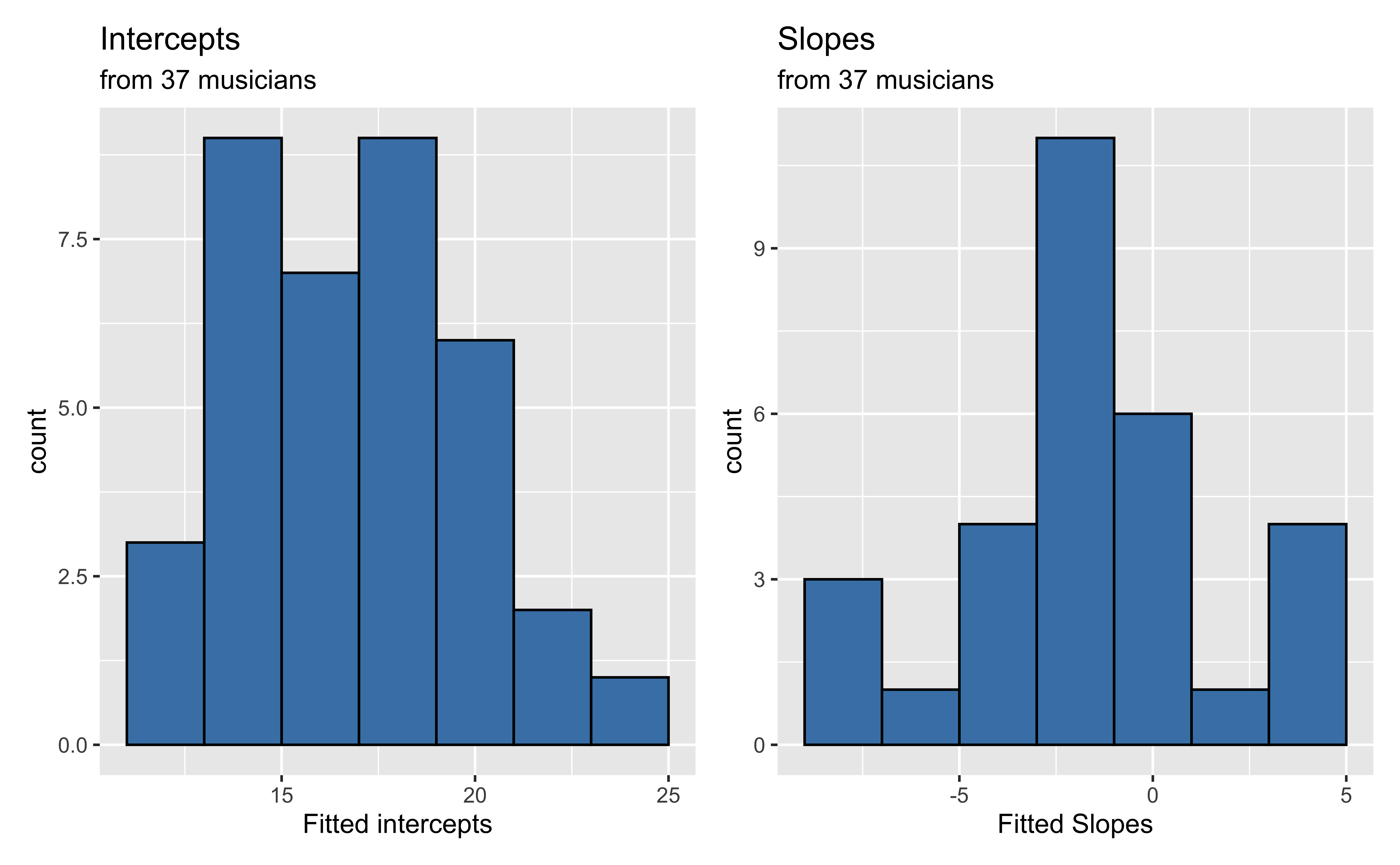
Recreated from BMLR Figure 8.9
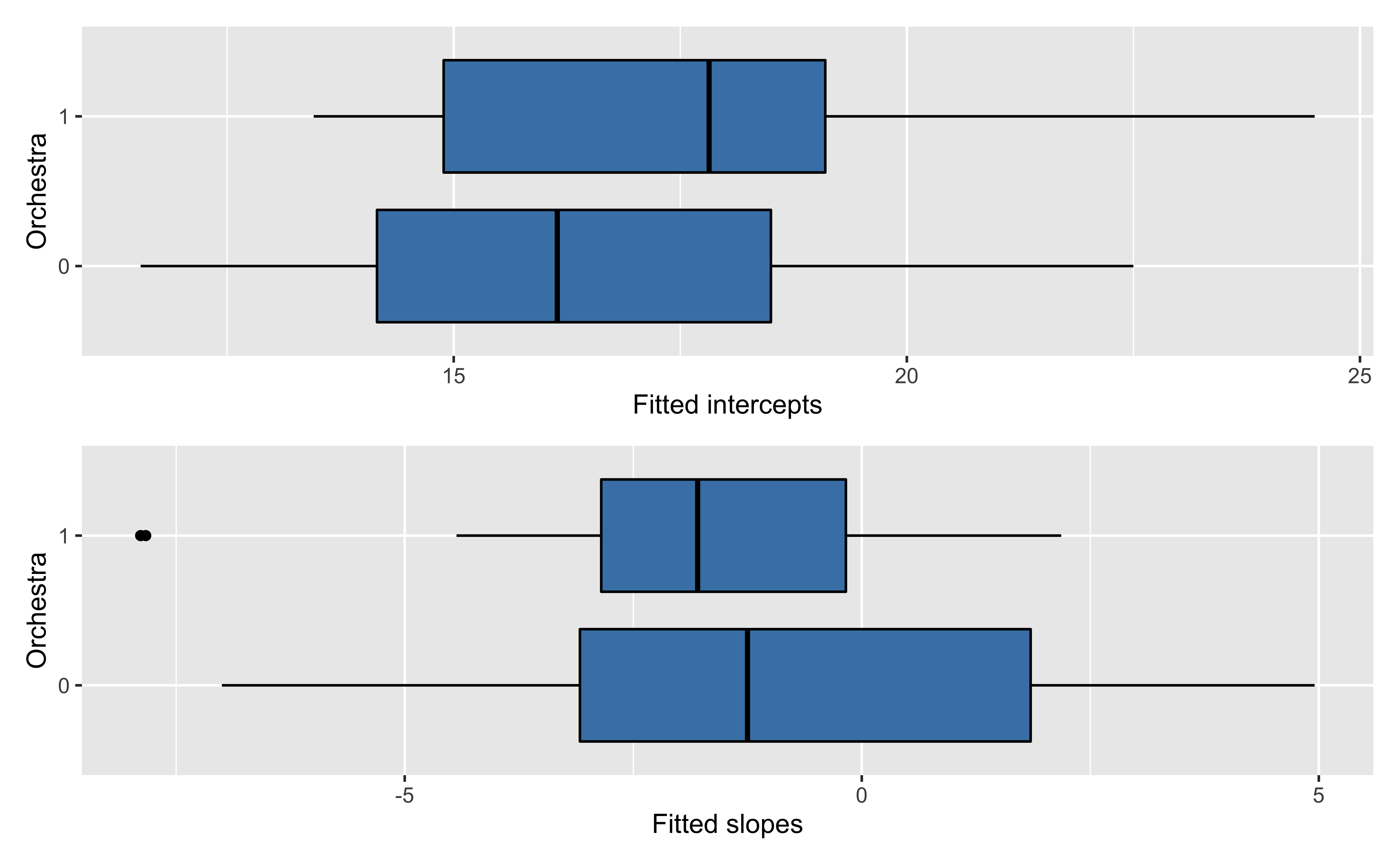
Now let’s consider if there is an association between the estimated slopes, estimated intercepts, and the type of instrument.
Level Two Model
The slope and intercept for the \(i^{th}\) musician can be modeled as
\[\begin{aligned}&a_i = \alpha_0 + \alpha_1 ~ Orchestra_i + u_i \\ &b_i = \beta_0 + \beta_1 ~ Orchestra_i + v_i\end{aligned}\]
Note the response variable in the Level Two models are not observed outcomes but the (fitted) slope and intercept from each musician
Application exercise
See Part 4: Level Two Models.
Estimated coefficients by instrument
Level Two model
Model for intercepts
| term | estimate | std.error | statistic | p.value |
|---|---|---|---|---|
| (Intercept) | 16.283 | 0.671 | 24.249 | 0.000 |
| orchestra | 1.411 | 0.991 | 1.424 | 0.163 |
Model for slopes
| term | estimate | std.error | statistic | p.value |
|---|---|---|---|---|
| (Intercept) | -0.771 | 0.851 | -0.906 | 0.373 |
| orchestra | -1.406 | 1.203 | -1.168 | 0.253 |
Writing out the models
Level One
\[\hat{na}_{ij} = \hat{a}_i + \hat{b}_i ~ LargeEnsemble_{ij}\]
for each musician.
Level Two
\[\begin{aligned}&\hat{a}_i = 16.283 + 1.441 ~ Orchestra_i \\ &\hat{b}_i = -0.771 - 1.406 ~ Orchestra_i\end{aligned}\]Composite model
\[\begin{aligned}\hat{na}_i &= 16.283 + 1.441 ~ Orchestra_i - 0.771 ~ LargeEnsemble_{ij} \\ &- 1.406 ~ Orchestra:LargeEnsemble_{ij}\end{aligned}\](Note that we also have the error terms \(\epsilon_{ij}, u_i, v_i\) that we will discuss next class.)
What is the predicted average performance anxiety before solos and small ensemble performances for vocalists and keyboardists? For those who place orchestral instruments?
What is the predicted average performance anxiety before large ensemble performances for those who play orchestral instruments?
Disadvantages to this approach
⚠️ Weighs each musician the same regardless of number of diary entries
⚠️ Drops subjects who have missing values for slope (7 individuals who didn’t play a large ensemble performance)
⚠️ Does not share strength effectively across individuals.
Application exercise
See Part 5: Distribution of \(R^2\) values.
Next time
We will use a unified approach that utilizes likelihood-based methods to address some of these drawbacks.
Acknowledgements
The content in the slides is from
Sadler, Michael E., and Christopher J. Miller. 2010. “Performance Anxiety: A Longitudinal Study of the Roles of Personality and Experience in Musicians.” Social Psychological and Personality Science 1 (3): 280–87. http://dx.doi.org/10.1177/1948550610370492.